Error Mitigation Overview

Error mitigation uses additional experiments, calibration or postprocessing to improve estimates from a noisy quantum device. Its usual target is a particular expectation value or probability. A better estimate does not necessarily correspond to a repaired quantum state, and lower bias can come with enough extra variance to make the estimate less accurate.

This overview develops that tradeoff, explains the main method families, and shows how calibration, rejected shots and method combinations affect the answer. The aim is to choose a procedure that estimates the same desired quantity more accurately at an acceptable cost (Cai et al., 2023).

Helpful background. Quantum measurement as estimation introduces estimators and loss. Variance and covariance explains uncertainty in combined data, and SPAM errors supplies the assumptions behind readout calibration.

Estimates, bias and statistical risk

Suppose the ideal circuit produces $\rho_\star$ and the desired number is

$\mu_\star=\operatorname{Tr}(O\rho_\star).$

An estimator $\widehat\mu$ is a function of the observed records, possibly including separate calibration data. For squared error,

$$\begin{aligned} \operatorname{Bias}(\widehat\mu)&=\mathbb E\widehat\mu-\mu_\star,\\ \operatorname{MSE}(\widehat\mu)&=\operatorname{Bias}^2+\operatorname{Var}(\widehat\mu). \end{aligned}$$

The expectation averages over repeated acquisitions, not over different physical targets unless an ensemble of tasks is explicitly specified. A single favorable realization does not determine either bias or MSE. The target should be fixed before choosing a method: changing from an unconditional mean to a postselected mean can change the scientific question.

Signed corrections can produce estimates outside the physical range of $O$. That is possible for a statistical estimator and is not a claim that a quantum state has an impossible expectation. Conversely, clipping estimates into a physical range changes their bias and uncertainty.

An exact bias–variance crossover

Consider independent outcomes $Y=\pm1$ with noisy mean $\mathbb E Y=\lambda\mu_\star$. Assume the attenuation $0<\lambda\leq1$ is known exactly. Compare the raw sample mean $\overline Y$ with the inverse estimate $\overline Y/\lambda$. Their risks at $N$ equal-cost shots are

$$\begin{aligned} R_{\rm raw}&=(1-\lambda)^2\mu_\star^2 +\frac{1-\lambda^2\mu_\star^2}{N},\\ R_{\rm inv}&=\frac{1-\lambda^2\mu_\star^2}{N\lambda^2}. \end{aligned}$$

The inverse is unbiased under this exact model, but has larger variance. For $\mu_\star=.6$, $\lambda=.8$,

$$\begin{aligned} R_{\rm raw}&=.0144+.7696/N,\\ R_{\rm inv}&=1.2025/N. \end{aligned}$$

Shots $N$	Raw MSE	Inverse MSE
$20$	$.052880$	$.060125$
$50$	$.029792$	$.024050$
$200$	$.018248$	$.006013$

Values are rounded to six decimals. Correction becomes better only for $N>30.0625$, hence integer $N\geq31$. The raw estimator approaches its squared-bias floor; the exact inverse keeps improving with more samples.

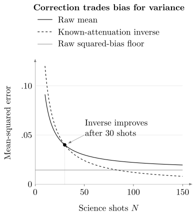
Exact risks for a binary observable with $\mu_\star=.6$ and known attenuation $\lambda=.8$. At small shot budgets the unbiased inverse is less accurate because of its extra variance. The gray horizontal line is the raw squared-bias floor $.0144$. Calibration uncertainty and its acquisition cost are excluded from this deliberately conditional comparison.

If attenuation must be learned, its calibration cost and uncertainty belong in the comparison. More science shots do not remove a fixed calibration error. This is why a method’s exact-model unbiasedness is useful but insufficient for predicting experimental accuracy.

What the main methods change

Method	How it obtains a different estimate
Readout correction	Uses a calibrated detector response to infer terminal probabilities or observables.
Zero-noise extrapolation	Runs related experiments at altered noise strengths and extrapolates to a specified zero-noise limit.
Probabilistic cancellation	Samples implementable noisy operations with signed weights representing the desired ideal operation.
Symmetry verification	Detects outcomes inconsistent with a promised ideal sector and uses a conditional or projected estimate.

Each method needs a physical or statistical assumption. Readout correction requires a response that applies to the science states and context. Extrapolation requires an appropriate family with the intended ideal limit; stretching or folding a circuit can also change coherent errors, leakage and timing. Cancellation requires the target operation to lie in the learned implementable span and the learned noise model to remain applicable. Symmetry checks miss errors within the accepted sector and can themselves be imperfect.

Temme, Bravyi and Gambetta (2017) gives foundational extrapolation and cancellation constructions. Symmetry-based filtering is developed by Bonet-Monroig et al. (2018); multiqubit detector corrections and their costs are studied by Bravyi et al. (2021). The linked specialist pages provide the detailed algorithms. Multiple-copy, learned and subspace-based estimators have further requirements; they do not inherit another method’s assumptions simply because both are called mitigation.

Dynamical decoupling and pulse recalibration change the physical experiment before inference. They can be combined with mitigation, but the improved raw experiment is then the relevant baseline. Quantum error correction protects encoded quantum information; fault tolerance also controls how faults spread through operations. Improvement of one terminal estimate alone establishes neither property. These approaches can coexist without answering the same question.

Signed weights and shot allocation

For fixed weights and a vector of measured means,

$$\begin{aligned} \widehat\mu&=\mathbf w^{\mathsf T}\widehat{\boldsymbol\mu},\\ \operatorname{Var}(\widehat\mu)&=\mathbf w^{\mathsf T}\Sigma\mathbf w. \end{aligned}$$

The covariance matrix must describe the actual acquisition. Shared calibration, paired random circuits and drift can correlate estimates. If the weights themselves are fitted, treating them as fixed omits their uncertainty and possible dependence on the measured means.

For means $(.71,.64)$, weights $(2,-1)$ and

$\Sigma=\begin{pmatrix}.0009&.0003\\.0003&.0016\end{pmatrix},$

the estimate is $.78$ and its variance is $.004$. Dropping covariance would give $.0052$. Positive covariance reduces variance here because the two weights have opposite signs; it would increase variance for two positive weights.

For independent component means, let a single shot at setting $i$ have variance $\sigma_i^2$ and cost $c_i>0$. With $n_i$ shots and total cost $T=\sum_i c_i n_i$, the continuous allocation optimum is

$$\begin{aligned} n_i&=\frac{T|w_i|\sigma_i/\sqrt{c_i}} {\sum_j|w_j|\sigma_j\sqrt{c_j}},\\ V_{\min}&=\frac{(\sum_i|w_i|\sigma_i\sqrt{c_i})^2}{T}. \end{aligned}$$

This assumes known variances, independent acquisitions and positive shot allocations for relevant noisy terms; finite integer budgets require rounding. Equal per-shot variances and equal costs reduce the relative variance scale to $\|\mathbf w\|_1^2$, with allocation proportional to $|w_i|$. That familiar factor is not a universal measured overhead: unequal variances, covariance, calibration and longer circuits change the comparison.

Calibration uncertainty and method combinations

If calibrated parameters $\widehat\theta$ enter an estimator $F$, a smooth local approximation adds

$V_{\rm cal}\simeq(\nabla_\theta F)^{\mathsf T}\Sigma_\theta\nabla_\theta F.$

There are also cross terms when science and calibration data are dependent. A small denominator, clipping or boundary constraints can make this approximation unreliable. Model mismatch is a possible bias, not merely another sample variance.

For the inverse example, $F=\overline Y/\widehat\lambda$ has leading calibration variance $\mu_\star^2\operatorname{Var}(\widehat\lambda)/\lambda^2$. Reusing the same calibration across observables creates shared uncertainty. It can lower the average acquisition cost, but averaging many science results does not average away that common error.

Combining methods defines a new estimator. Correcting a full outcome distribution and then selecting a sector generally differs from discarding outcomes first and correcting the remainder. The discarded outcomes can include valid states misclassified by the detector, while retained outcomes can include contamination from other sectors. Exercise6 gives a finite example.

Likewise, physical suppression can change the detector or noise model needed by a later correction, and extrapolation can change symmetry acceptance. Check the complete ordered procedure on tasks not used to choose its settings. Selecting a polynomial order, clipping threshold or method using the same data later presented as an independent test gives an overly favorable comparison. Device characterization and algorithmic benchmarking discuss these experimental comparisons.

Postselection changes both the target and the cost

For an acceptance event $A$ and recorded observable $O$, distinguish

$$\begin{aligned} a&=\Pr(A),\\ \mu_A&=\mathbb E[O|A],\\ x_A&=\mathbb E[O\mathbf1_A]=a\mu_A. \end{aligned}$$

Neither accepted quantity automatically equals the original ideal target. In a projective sector check with projector $P$, a subsequent observable measurement instead has conditional expectation

$\mu_P=\frac{\operatorname{Tr}(POP\rho)}{\operatorname{Tr}(P\rho)}.$

This is a well-defined projected-state expectation for positive acceptance. Inferring it by jointly reading an observable and a symmetry requires a compatible measurement scheme; noncommuting checks can disturb the state. A promised ideal sector also does not ensure that filtering improves every noisy expectation—errors within the sector remain.

Among $1000$ attempts, suppose accepted records contain $420$ plus and $180$ minus outcomes, while rejected records contain $260$ plus and $140$ minus. Then $a=.6$, $\mu_A=.4$, and $x_A=.24$. The full observed mean is $.36$, a fourth quantity. None of these arithmetic facts tells us the unknown ideal value.

For $N$ independent stationary attempts, the accepted count $K$ is binomial. Conditional on $K>0$, the variance of the accepted sample mean is

$\sigma_A^2\mathbb E[1/K\mid K>0],$

where $\sigma_A^2=\operatorname{Var}(O|A)$. Replacing the reciprocal expectation by $1/(Na)$ is a large-count approximation, not an exact identity. The chance of no accepted sample is $(1-a)^N$.

Alternatively, stop after obtaining a fixed $r$ accepted samples. Under the same independent stationary assumptions, the attempted count has mean $r/a$ and variance $r(1-a)/a^2$. Rejected attempts still consume preparation and measurement time. Temporal correlations, drift or adaptive acceptance require a different sampling analysis.

Choosing a useful procedure

Compare the same target at equal total resources, or compare the cost of attaining the same accuracy and confidence. Include calibration, rejected attempts, extra settings, circuit duration and classical processing. A comparison at equal science-shot count can be informative, but it is conditional on those other costs rather than a complete resource comparison.

Use exactly calculable small circuits, analytic limits or independently bounded references to test predictions. Agreement with values generated by the same fitted noise model checks internal consistency, not robustness to model error. Report improvements and failures across the intended range of circuits; one favorable observable is not a general guarantee.

Noise can erase information needed to distinguish ideal outputs. Recovering those distinctions uniformly can force a large sampling cost, even for elaborate postprocessing (Takagi, Tajima and Gu, 2023). Limits of error mitigation explains the hypotheses of such bounds. They do not make every finite mitigation task useless, and a successful finite example does not establish scalable protection of deep computations. When weights, acceptance or calibration stability make the requested precision impractical, improving controls, changing the experiment or using encoded protection can be the more effective choice.

Exercises

1. Find the shot-budget crossover

Derive the two exact risks for the binary attenuation model and find when inverse correction improves the example $\mu_\star=.6,\lambda=.8$.

Solution

Since $Y^2=1$, its variance is $1-\lambda^2\mu_\star^2$. The raw mean has bias $(\lambda-1)\mu_\star$ and variance divided by $N$. Division by known $\lambda$ removes the bias and multiplies variance by $1/\lambda^2$. Their risk difference is $.4329/N-.0144$, so correction is better when $N>30.0625$. For a target exactly zero, the raw estimator already has zero bias; this inverse only increases variance. The comparison is target-dependent.

2. Allocate shots with unequal costs

Minimize $\sum_i w_i^2\sigma_i^2/n_i$ at fixed $\sum_i c_i n_i=T$. Evaluate the result for $w=(2,-1)$, $\sigma=(.6,.8)$ and $c=(1,4)$.

Solution

A Lagrange multiplier gives $n_i=|w_i|\sigma_i/\sqrt{\nu c_i}$. Imposing the cost constraint gives the allocation in the text. Here the weighted sum is $2(.6)+(.8)\sqrt4=2.8$, so $n_1=3T/7$, $n_2=T/7$ and $V_{\min}=7.84/T$. The second setting gets fewer shots because each costs four times as much. Integer rounding matters for small $T$.

3. Reuse a finite calibration

At $\lambda=.8$, a trusted reference with ideal mean one is measured $M$ times to estimate $\lambda$. For the target $.6$, find the leading calibration variance of inverse correction and explain its correlation across repeated science batches.

Solution

Reference outcomes are $\pm1$, so $\operatorname{Var}(\widehat\lambda)=.36/M$. The correction derivative at the mean is $-\mu_\star/\lambda=-.75$, giving $V_{\rm cal}\simeq.2025/M$. Two independent science batches using this same calibration share this leading covariance. Averaging the batches reduces their independent shot noise but leaves the common calibration contribution. This is a local approximation; random-denominator bias and rare small denominators require attention for small $M$.

4. Filtering can worsen an observable

In a three-level system let $\rho=\operatorname{diag}(.4,.2,.4)$, $P=\operatorname{diag}(1,1,0)$ and $O=\operatorname{diag}(1,-1,1)$. The ideal target is $|0\rangle$, which lies in $P$. Compare the raw and projected expectations.

Solution

The target expectation is one. The raw value is $.4-.2+.4=.6$. Acceptance is $.6$ and the projected expectation is $(.4-.2)/.6=1/3$, farther from the target. The accepted sector contains erroneous population in $|1\rangle$, while the rejected state’s observable value happened to agree with the target. A valid ideal-sector promise does not imply monotone improvement of each observable.

5. Count attempts and zero-acceptance runs

At acceptance $a=.6$, find the expected attempts and their variance to obtain $r=5000$ accepted samples. For a different low-yield experiment with $a=.1$ and exactly $N=10$ attempts, find the probability of no accepted sample.

Solution

The stopping-rule mean is $5000/.6\simeq8333.333$ attempts and its variance is $5000(.4)/(.6)^2\simeq5555.556$. Expected rejected attempts are approximately $3333.333$. The low-yield fixed-budget experiment has probability $.9^{10}\simeq.348678$ of no accepted sample, so a conditional mean is not even defined in more than a third of runs. Fixed attempted and fixed accepted budgets are different experiments.

6. Correcting and selecting do not commute

Use latent probabilities $\mathbf p=(.6,.3,.1)^{\mathsf T}$ and column-stochastic response

$A=\begin{pmatrix}.8&.1&.1\\.1&.8&.2\\.1&.1&.7\end{pmatrix}.$

The desired conditional probability is for latent outcome zero among outcomes zero and one. Compare full response correction followed by conditioning with discarding reported outcome two first and inverting only the upper-left block.

Solution

The observed vector is $(.52,.32,.16)^{\mathsf T}$. Full inversion recovers $\mathbf p$, giving $.6/(.6+.3)=2/3$. Inverting the retained block on $(.52,.32)^{\mathsf T}$ instead gives $(64/105,34/105)^{\mathsf T}$. Renormalizing yields $32/49\simeq.653061$, not $2/3$. Normalizing the retained observed data first gives the same final wrong ratio. This block inverse ignores contamination from latent outcome two. If the full response and absolute retained probabilities are known, normalization can supply the third observed probability; that is a full-model reconstruction, not inversion of the truncated block.

7. Account for a complete finite comparison

A method uses $8000$ science attempts, $1500$ calibration attempts and $500$ validation attempts; exactly $75\%$ of science records are accepted. What should be compared with a raw procedure given $10{,}000$ attempts?

Solution

The method uses $10{,}000$ attempts in total and retains $6000$ science records. Compare estimates of the same target using those complete budgets, preserving calibration uncertainty and the effect of rejection. Equal attempt count still does not imply equal duration if transformed circuits are longer, nor equal classical processing cost. If calibration is reused, state the workload across which its cost is divided and test that it remains applicable. A numerical improvement on this comparison describes that task and budget, not an automatic improvement of every state or future computation.

References

• X. Bonet-Monroig, R. Sagastizabal, M. Singh, and T. E. O’Brien, “Low-cost error mitigation by symmetry verification,” Physical Review A 98, 062339 (2018), doi:10.1103/PhysRevA.98.062339.
• S. Bravyi, S. Sheldon, A. Kandala, D. C. McKay, and J. M. Gambetta, “Mitigating measurement errors in multiqubit experiments,” Physical Review A 103, 042605 (2021), doi:10.1103/PhysRevA.103.042605.
• Z. Cai, R. Babbush, S. C. Benjamin, S. Endo, W. J. Huggins, Y. Li, J. R. McClean, and T. E. O’Brien, “Quantum error mitigation,” Reviews of Modern Physics 95, 045005 (2023), doi:10.1103/RevModPhys.95.045005.
• R. Takagi, H. Tajima, and M. Gu, “Universal sampling lower bounds for quantum error mitigation,” Physical Review Letters 131, 210602 (2023), doi:10.1103/PhysRevLett.131.210602.
• K. Temme, S. Bravyi, and J. M. Gambetta, “Error mitigation for short-depth quantum circuits,” Physical Review Letters 119, 180509 (2017), doi:10.1103/PhysRevLett.119.180509.