Markovian and Non-Markovian Noise

A quantum channel predicts the result of one input–output experiment. Predicting a sequence requires more: how the noise changes with time, what the apparatus retains between operations, and how an intermediate measurement or reset affects the future. Different meanings of “Markovian” answer different parts of this question.

This page compares fixed-step channel powers, continuous semigroups, CP divisibility and experiments that interrupt the evolution. The calculations use finite-dimensional systems and a common preparation procedure. Formal definitions and broader open-system theory are developed in what non-Markovian means.

Helpful background. Quantum channels supplies composition and Choi matrices. SPAM errors explains why preparation, detector calibration and drift matter when comparing experiments at different times.

Channel composition across time

Write the reduced evolution from the original preparation as

$\rho(t)=\Phi_{t:0}[\rho(0)].$

A collection of CPTP maps $\Phi_{t:0}$ gives terminal predictions. It does not automatically specify what happens if a new state is prepared at time $s$, or if a measurement is inserted there. Nor does physicality of every terminal map guarantee a CPTP factorization

$\Phi_{t:0}=V_{t:s}\circ\Phi_{s:0}.$

The following conditions make progressively different demands, rather than forming one universal ladder:

Condition	Mathematical question
Fixed-step powers	Does $\Phi_{n\Delta:0}=\Phi_{\Delta:0}^{n}$ hold at the tested endpoints?
CP divisibility	Does a CPTP $V_{t:s}$ exist for every ordered pair of times?
Time-homogeneous semigroup	Does a continuous family satisfy $\Phi_{t+s}=\Phi_t\circ\Phi_s$, with $\Phi_0=\mathrm{id}$?
Operational absence of memory	After the same system replacement, do future statistics depend on earlier operations or outcomes?

A semigroup gives CP divisibility through $V_{t:s}=\Phi_{t-s}$, but the converse fails. Fixed powers only constrain a sampled grid and need not embed into a continuous semigroup. Even exact agreement of uninterrupted terminal maps with a semigroup does not determine all intervention statistics.

In particular, agreement with $\Phi_\Delta^n$ does not establish that the same conditional transformation acts after every possible history. The two-step example below passes this endpoint test while retaining information that a measurement and reset reveal.

The system being modeled matters. A qubit may have memory through a retained resonator or spectator; the enlarged system can still have a simple state-update law. Initial correlations can also prevent a single preparation-independent CPTP map from applying to arbitrary system inputs. Keep those degrees of freedom or specify the restricted preparation family.

Nonexponential decay can be CP-divisible

For real $|\eta|\leq1$, qubit dephasing acts as

$$\mathcal D_\eta\begin{pmatrix}a&b\\c&d\end{pmatrix} =\begin{pmatrix}a&\eta b\\\eta c&d\end{pmatrix}.$$

The factors multiply under composition. The exponential envelope $\eta_E(t)=e^{-\gamma t}$, with $\gamma\geq0$, therefore gives a semigroup. The Gaussian envelope $\eta_G(t)=e^{-(t/\tau)^2}$ does not: the square of $s+t$ contains a cross term absent from $s^2+t^2$.

Nevertheless, for every finite $t\geq s\geq0$,

$\frac{\eta_G(t)}{\eta_G(s)}=e^{-(t^2-s^2)/\tau^2}\in(0,1].$

This ratio defines a CPTP dephasing propagator, so the family is CP-divisible. Its time-local equation is

$$\begin{aligned} \dot\rho&=\frac{\kappa(t)}2(Z\rho Z-\rho),\\ \kappa(t)&=\frac{2t}{\tau^2}\geq0. \end{aligned}$$

Take $\gamma=.5$, $\tau=2$ and time in consistent units. Rounded to six decimals:

Envelope	$\eta(1)$	$\eta(2)$	$\eta(1)^2$
Exponential	$0.606531$	$0.367879$	$0.367879$
Gaussian	$0.778801$	$0.367879$	$0.606531$

The shared endpoint at $t=2$ cannot distinguish these laws. The Gaussian law fails fixed repetition of its first interval, but its later interval factor is $e^{-3/4}\simeq0.472367$ and remains physical.

A nonnegative-rate equation specifies this reduced-map family, not a unique multitime experiment. For example, static Gaussian detuning and a time-dependent dephasing model can have the same Gaussian envelope but different echo responses; see the worked comparison in dephasing and amplitude damping.

Intermediate maps and singular times

CP divisibility is an existence condition. If $\Phi_{s:0}$ is invertible as a linear superoperator, the only candidate is

$V_{t:s}=\Phi_{t:0}\circ\Phi_{s:0}^{-1}.$

The inverse need not itself be positive. Test the complete candidate, not its individual factors. With output-first ordering and normalized maximally entangled state $|\Omega\rangle=d^{-1/2}\sum_j|j\rangle|j\rangle$, define

$$\begin{aligned} J_N(V)&=(V\otimes\mathrm{id})(|\Omega\rangle\langle\Omega|),\\ J_N(V)&\succeq0,\qquad\operatorname{Tr}_{\rm out}J_N(V)=I/d. \end{aligned}$$

Both positivity and the partial-trace condition are required. This $J_N$ is the unnormalized Choi matrix used in channel representations divided by input dimension $d$.

For dephasing with $\eta(s)\ne0$, the candidate is $\mathcal D_r$ with $r=\eta(t)/\eta(s)$. Its normalized Choi matrix is

$$J_N(\mathcal D_r)=\frac12 \begin{pmatrix}1&0&0&r\\0&0&0&0\\0&0&0&0\\r&0&0&1\end{pmatrix}.$$

Its eigenvalues are $(1-r)/2,(1+r)/2,0,0$. Thus it is CPTP exactly when $|r|\leq1$. Terminal factors $\eta(1)=.4$ and $\eta(2)=.7$ are individually physical, but their interval ratio $1.75$ gives eigenvalues $-.375,1.375,0,0$: a trace-preserving but non-CP candidate.

At $\eta(s)=0$, division is unavailable. If every later factor stays zero, many propagators work on the diagonal image—for example the identity and complete dephasing both preserve it. If coherence later revives, no linear propagator exists: earlier evolution maps $|+\rangle$ and $|-\rangle$ to the same $I/2$, whereas the later map separates them again.

More generally, factorization requires

$\ker\Phi_{s:0}\subseteq\ker\Phi_{t:0}.$

This guarantees a well-defined linear map on the earlier image, but does not by itself give a CPTP extension to the full space. Singular cases require an existence problem, not an arbitrary pseudoinverse (Chruściński, Rivas and Størmer, 2018). Near singularity, inversion also amplifies uncertainty in tomography; a small negative estimated eigenvalue needs uncertainty analysis before being interpreted.

What distinguishability and rate tests establish

For two consistently prepared inputs,

$D(t)=\tfrac12\|\Phi_{t:0}(\rho_1-\rho_2)\|_1.$

Every positive trace-preserving propagator contracts this distance. A resolved increase therefore rules out P divisibility and hence CP divisibility for the common map family. For $|+\rangle,|-\rangle$ under dephasing, $D(t)=|\eta(t)|$; the preceding example revives by $.3$. This is the trace-distance test of Breuer, Laine and Piilo (2009).

The converse is false: even absence of revival for every system-state pair does not establish CP divisibility. Exercise6 gives an explicit Pauli-channel example. A finite selection of pairs and sample times is weaker still. Ancilla-assisted tests can probe complete positivity, but a formal Choi input at an intermediate time need not be reachable by an uninterrupted experiment from the original preparation.

For a differentiable, invertible finite-dimensional family, nonnegative rates in a canonical time-local generator characterize CP divisibility. The qualification “canonical” matters: an arbitrary redundant operator expansion can include negative coefficients even for a positive-rate generator. At singular times rates can diverge or become nonunique. CP divisibility and non-Markovianity measures develop the general theory.

Identical terminal channels, different behavior after reset

Here is a complete two-step model with a classical memory. Each interval applies either $I$ or $X$. Write the bit-flip channel as

$\mathcal X_p(\rho)=(1-p)\rho+pX\rho X.$

In model M, the interval faults $E_1,E_2$ are independent Bernoulli variables with probability $p=.1$. The cumulative flips are $B_1=E_1$ and $B_2=E_1\mathbin{\mathrm{xor}}E_2$.

In model C, sample independent variables $L$ and $C_2$ with probabilities $p=.1$ and $q=2p(1-p)=.18$. Apply faults $E_1=L$ and $E_2=L\mathbin{\mathrm{xor}}C_2$. Retain $L$ between intervals. Without an intervention, cancellation gives $B_1=L$ and $B_2=C_2$.

Both models produce $\mathcal X_{.1}$ after step one and $\mathcal X_{.18}=\mathcal X_{.1}^2$ after step two, for every initial state. Their endpoint maps therefore pass the same fixed-power test. Now start in $|0\rangle$, measure $Z$ after step one to obtain $B_1$, and reprepare $|0\rangle$ regardless of that result. Leave the classical fault variables untouched. The next $Z$ outcome equals $E_2$:

First result $B_1$	Model M: next result $1$	Model C: next result $1$
$0$	$.10$	$.18$
$1$	$.10$	$.82$

Both branches have nonzero probability. The different conditional predictions expose memory that endpoint tomography misses.

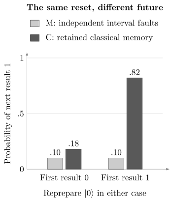
The two models have identical uninterrupted channels at both sampled times. After measuring and repreparing $|0\rangle$, the independent model gives the same future probability for either earlier result. The retained-memory model gives $.18$ or $.82$. Resetting the system does not reset its classical environment.

This measurement-and-repreparation is a causal break: the outgoing system state is fixed, so a dependence of later statistics on past results must be carried elsewhere, provided the replacement operation and future controls are indeed the same. A general operational Markov condition requires independence for all suitable past operations, break outcomes and replacement states (Pollock et al., 2018). A restricted experiment can reveal memory without ruling out every untested form when it sees none.

The relevant object is a process tensor: it predicts final states or outcome probabilities for sequences of interventions. A family of one-time channels does not supply those temporal correlations. What non-Markovian means introduces this distinction, and collision models gives explicit environmental constructions.

Designing an informative comparison

Compare a channel estimated from one-step experiments with new sequence lengths, rather than fitting a new channel independently at every length and calling that agreement. Use preparations and measurements sensitive to the directions being predicted. For continuous-time claims, include unequal interval lengths; a sampled power law alone cannot test all partitions.

Interleave different sequences in acquisition time. Otherwise long circuits measured later can confuse elapsed laboratory time with circuit history. Vary gate identities at matched duration, spectator activity, leakage-resolving readout and reset procedures. Fixed-step failure can reflect known time dependence, gate dependence, control distortion or an inadequate SPAM model; it does not uniquely identify an environment. Proctor et al. (2020) discusses time-resolved drift tests.

A useful test asks whether an earlier change affects later outcomes after the same replacement state, with unchanged later settings. Retaining a resonator, spectator, leaked level or classical controller state may then give a simpler enlarged model. Such a model can predict well without uniquely identifying the microscopic cause. Device characterization covers experiment design; noise simulation covers explicit state and history propagation.

Exercises

1. A fixed channel need not embed into a semigroup

A qubit Pauli channel has probabilities $(p_I,p_X,p_Y,p_Z)=(.3,.3,.3,.1)$. Find its Bloch multipliers and show that no finite time-independent Hermiticity-preserving generator can exponentiate to this map.

Solution

Conjugation by a Pauli preserves its own axis and reverses the other two. The multipliers are $(.2,.2,-.2)$, so the real Pauli transfer matrix is $\operatorname{diag}(1,.2,.2,-.2)$ with determinant $-.008$. For a real finite generator $L$, $\det e^{tL}=e^{t\operatorname{Tr}L}>0$. This rules out a time-independent continuous embedding, including a GKSL semigroup. The finite map and all its integer powers remain CPTP. The obstruction addresses this embedding, not every possible time-dependent implementation.

2. Compare exponential and Gaussian intervals

Calculate the table above and prove CP divisibility of the Gaussian family without assuming time homogeneity.

Solution

At $\gamma=.5,\tau=2$, the exponential factors are $e^{-1/2}$ and $e^{-1}$, while the Gaussian factors are $e^{-1/4}$ and $e^{-1}$. Squaring the first Gaussian factor gives $e^{-1/2}$, differing from its true second endpoint by approximately $.238651$.

For any ordered pair $t\geq s$, the ratio is $e^{-(t^2-s^2)/4}\leq1$ and positive, so it defines a CPTP dephasing map. These ratios also compose consistently across three times. They depend on both endpoints, not just the interval length. This proves divisibility of the specified family, not absence of memory under arbitrary inserted controls.

3. Test a revival and an erased direction

Find the interval Choi spectrum for $.4\to.7$ dephasing. Then explain why $0\to.7$ cannot factor through any linear system map.

Solution

The invertible case has ratio $r=7/4$ and normalized Choi spectrum $(-3/8,0,0,11/8)$. The output partial trace remains $I/2$, but positivity fails. For the singular case, complete dephasing erases $X$, whereas the later map sends $X$ to $.7X$. The required kernel inclusion fails. No choice of extension or pseudoinverse can restore the lost preparation-dependent distinction.

4. Derive the trace-distance witness

Use the dephased plus and minus states to derive $D(t)$ and state what an increase establishes.

Solution

The initial difference is $X$. Its evolved eigenvalues are $\pm\eta(t)$, giving half the trace norm $D(t)=|\eta(t)|$. The example grows from $.4$ to $.7$. Since a positive TP map contracts trace distance between states, this excludes a positive TP interval propagator and therefore excludes a CPTP one. The comparison assumes the same preparations and detector model at both times; changing those would change the experiment being compared.

5. Calculate the causal-break predictions

Enumerate both two-step fault models, their cumulative joints, and their future conditionals after the replacement. Compare the covariance of cumulative flips with the memory test.

Solution

In order $(B_1B_2)=(00,01,10,11)$,

$$\begin{aligned} \mathbf p_M&=(.81,.09,.01,.09),\\ \mathbf p_C&=(.738,.162,.082,.018). \end{aligned}$$

Both have first-flip probability $.1$ and cumulative second-flip probability $.18$. Their total-variation distance is $.144$. The cumulative covariance is $.09-(.1)(.18)=.072$ in M and zero in C: cumulative variables can be correlated even for independent increments.

After replacement, the future result is the interval fault $E_2$. In M it has probability $.1$ independently of $B_1$. In C, $E_2=L\mathbin{\mathrm{xor}}C_2$ gives $.18$ for $L=0$ and $.82$ for $L=1$. Zero cumulative covariance therefore does not establish absence of operational memory.

6. No system-state revival, but failure of CP divisibility

In dimensionless time, consider Pauli multipliers

$\lambda_x(t)=\lambda_y(t)=\frac{1+e^{-2t}}2,\qquad\lambda_z(t)=e^{-2t}.$

Show that terminal maps are CPTP and every system-state trace distance decreases, yet intermediate maps are non-CP for $t>s>0$ (Hall et al., 2014).

Solution

The Pauli probabilities are $p_I=(1+e^{-2t})/2$, $p_X=p_Y=(1-e^{-2t})/4$ and $p_Z=0$, hence all terminal maps are CPTP. For a Bloch-vector difference $\delta\mathbf r$, trace distance is $\tfrac12\sqrt{\sum_j\lambda_j(t)^2\delta r_j^2}$. Each positive multiplier decreases, so every such distance does too.

Put $u=e^{-2s}$ and $v=e^{-2t}$, with $0<v<u<1$. The unique interval has transverse multiplier $(1+v)/(1+u)$ and longitudinal multiplier $v/u$. Its would-be $Z$ probability, an eigenvalue of the normalized Choi matrix, is

$p_Z^{\rm int}=-\frac{(u-v)(1-u)}{4u(1+u)}<0.$

Thus absence of all system-only trace-distance revivals is weaker than CP divisibility. In the convention $\dot\rho=\tfrac12\sum_j\gamma_j(\sigma_j\rho\sigma_j-\rho)$, this family has $\gamma_x=\gamma_y=1$ and $\gamma_z=-\tanh t$; the negative canonical rate agrees with the intermediate-map calculation.

7. A negative displayed coefficient need not be a negative canonical rate

Let $\mathcal D_Z(\rho)=Z\rho Z-\rho$. Explain why writing $\mathcal L=2\mathcal D_Z-\mathcal D_Z$ does not make $e^{t\mathcal L}$ non-CP-divisible.

Solution

The two terms use the same operator and combine to $\mathcal L=\mathcal D_Z$. Its coherence factor is $e^{-2t}$ and all interval factors lie in $(0,1]$. The minus sign appeared only because the expansion was redundant. Canonical rates come from diagonalizing the decoherence matrix in a linearly independent orthonormal operator basis, after separating the Hamiltonian part. Coefficients in an arbitrary expansion do not have that invariant interpretation.

References

• H.-P. Breuer, E.-M. Laine, and J. Piilo, “Measure for the degree of non-Markovian behavior of quantum processes in open systems,” Physical Review Letters 103, 210401 (2009), doi:10.1103/PhysRevLett.103.210401.
• H.-P. Breuer, E.-M. Laine, J. Piilo, and B. Vacchini, “Colloquium: Non-Markovian dynamics in open quantum systems,” Reviews of Modern Physics 88, 021002 (2016), doi:10.1103/RevModPhys.88.021002.
• D. Chruściński, Á. Rivas, and E. Størmer, “Divisibility and information flow notions of quantum Markovianity for noninvertible dynamical maps,” Physical Review Letters 121, 080407 (2018), doi:10.1103/PhysRevLett.121.080407.
• M. J. W. Hall, J. D. Cresser, L. Li, and E. Andersson, “Canonical form of master equations and characterization of non-Markovianity,” Physical Review A 89, 042120 (2014), doi:10.1103/PhysRevA.89.042120.
• F. A. Pollock, C. Rodríguez-Rosario, T. Frauenheim, M. Paternostro, and K. Modi, “Non-Markovian quantum processes: Complete framework and efficient characterization,” Physical Review A 97, 012127 (2018), doi:10.1103/PhysRevA.97.012127.
• F. A. Pollock, C. Rodríguez-Rosario, T. Frauenheim, M. Paternostro, and K. Modi, “Operational Markov condition for quantum processes,” Physical Review Letters 120, 040405 (2018), doi:10.1103/PhysRevLett.120.040405.
• T. Proctor, M. Revelle, E. Nielsen, K. Rudinger, D. Lobser, P. Maunz, R. Blume-Kohout, and K. Young, “Detecting and tracking drift in quantum information processors,” Nature Communications 11, 5396 (2020), doi:10.1038/s41467-020-19074-4.