Device Characterization

Device characterization uses experiments to learn a predictive model of a quantum device. A Ramsey trace may reveal detuning; measurements with a neighboring qubit in different states may reveal a coupling. The central question is whether the chosen experiments distinguish the proposed explanations. A precise fit is useful only within a model that predicts other observations.

Required background. Rabi and Ramsey control introduces driven-qubit experiments; quantum noise distinguishes channels and fluctuations. Process tomography explains channel reconstruction and randomized benchmarking explains ensemble performance measurements.

Identifying a frequency from Ramsey measurements

Prepare $|+\rangle$, evolve under $H=\hbar\Delta Z/2$, and measure along $X$ or $Y$. Here $\Delta$ is angular-frequency detuning relative to the control reference. With ideal axes, a visibility $V$, an initial phase $\phi$ and an exponential envelope, the probabilities of the positive outcomes are

$$\begin{aligned} p_X(t)&=\frac{1+Ve^{-\gamma t}\cos\theta(t)}2,\\ p_Y(t)&=\frac{1+Ve^{-\gamma t}\sin\theta(t)}2,\\ \theta(t)&=\Delta t+\phi. \end{aligned}$$

These signs specify the analysis convention; a pulse-based implementation must translate its outcome labels accordingly. The exponential is an assumption to test, not part of the definition of Ramsey interferometry.

Measuring only $X$ cannot distinguish $(\Delta,\phi)$ from $(-\Delta,-\phi)$. Adding $Y$ distinguishes the phase direction. However, one evolution time still determines only $\Delta t+\phi$: measuring more quadratures at that same time cannot separate an unknown detuning from an unknown initial phase.

Multiple times help, but the time grid matters. At $t=m\tau$, every integer $k$ gives the same two-quadrature data for

$$\Delta' =\Delta+\frac{2\pi k}{\tau}.$$

This is frequency aliasing. More shots at those same times cannot remove it. A justified prior frequency interval or additional times that distinguish the candidate aliases are needed.

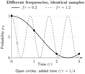
With $V=1$, $\gamma=\phi=0$, frequencies $f\tau=0.2$ and $1.2$ give identical $X$ probabilities at every integer $t/\tau$. The same alias survives $Y$ measurements. An added time $t/\tau=1/4$ separates these two candidates, although a broader frequency range can contain other aliases.

The fitted visibility can also be ambiguous. If preparation has transverse Bloch length $c$ and symmetric readout has contrast $v$, these experiments see only $V=cv$. Pairs $(c,v)=(0.8,1)$ and $(1,0.8)$ predict the same record. An independent preparation or detector measurement is needed to attribute the contrast loss. Degen, Reinhard and Cappellaro discuss how experimental design converts such phase information into parameter estimates.

Counts, sensitivity and prediction

For independent shots at fixed settings, the number of positive outcomes is binomial:

$$n_x\sim\operatorname{Binomial}(N_x,p_\theta(x)).$$

The log likelihood, apart from constants, is

$$\ell(\theta)=\sum_x n_x\log p_\theta(x) +\sum_x(N_x-n_x)\log(1-p_\theta(x)).$$

A likelihood fit respects the probability-dependent sampling variance. Ordinary least squares with constant error bars can be inappropriate near probabilities zero or one. Correlated shots, drifting parameters or uncertain calibration need an expanded likelihood or a valid analysis of correlated data.

The Jacobian $J_{xa}=\partial p_\theta(x)/\partial\theta_a$ describes local sensitivity. In a regular model its rank identifies the parameter combinations accessible to first order. A singular Jacobian need not prove global nonidentifiability in every nonlinear model; it can also mark a special point with vanishing first-order sensitivity. Conversely, full rank near one fit does not exclude distant aliases. Confidence regions should retain multiple plausible solutions when the experiment cannot distinguish them.

Predictions reveal different failures depending on what is held out:

New data	What it tests	What it does not establish
More shots of the same circuits	Sampling predictions in those settings	New-circuit behavior
New lengths or pulse orders	Composition and history dependence	Stability at a later date
Different spectator states	Transfer between contexts	Every many-qubit configuration
A later acquisition period	Stability over that period	Permanent stationarity

Compare predictions with the actual counts. For example, a model predicting $p=0.50$ with $N=1000$ gives a shot-noise scale $\sqrt{0.25/1000}\approx0.0158$ for the observed frequency. A residual of $0.10$ is about $6.32$ such scales. It suggests a failed prediction if the data were held out and independent; it is not automatically a universal significance calculation after fitting many parameters or searching many residuals.

Coherent rotations and irreversible noise

A constant unwanted rotation $U_\epsilon=e^{-i\epsilon Z/2}$ has average infidelity

$$r=\frac23\sin^2(\epsilon/2)\approx\frac{\epsilon^2}{6}.$$

The same commuting error repeated $m$ times rotates by $m\epsilon$. Phase-sensitive sequences can therefore reveal a signed error hidden by a small one-gate infidelity. Target/inverse sequences must be chosen carefully: some error terms cancel rather than amplify.

A trace-preserving qubit channel acts affinely on Bloch vectors:

$$\boldsymbol r'=T\boldsymbol r+\boldsymbol t.$$

It is unital precisely when $\boldsymbol t=0$. Unitary evolution rotates the Bloch ball; nonunitary evolution can contract and translate it. Amplitude damping can even increase the purity of some inputs by moving them toward the ground state. Purity loss is therefore not a universal definition of irreversible noise.

Wallman and colleagues define unitarity using the traceless transfer block. For a qubit,

$$u=\frac13\operatorname{Tr}(T^{\mathsf T}T).$$

A unitary channel has $u=1$; a depolarizing channel $T=pI$ has $u=p^2$. A complete reset to $|0\rangle$ has pure outputs but $T=0$, hence $u=0$. This removes the misleading contribution of nonunital translation. Unitarity adds information to average fidelity, but does not specify a unique microscopic mechanism or a literal fraction of coherent errors.

A fitted contraction must still be physical

For a Pauli-diagonal unital qubit map with diagonal entries $(\lambda_x,\lambda_y,\lambda_z)$, the four Pauli probabilities are

$$\begin{aligned} p_I&=(1+\lambda_x+\lambda_y+\lambda_z)/4,\\ p_X&=(1+\lambda_x-\lambda_y-\lambda_z)/4,\\ p_Y&=(1-\lambda_x+\lambda_y-\lambda_z)/4,\\ p_Z&=(1-\lambda_x-\lambda_y+\lambda_z)/4. \end{aligned}$$

Complete positivity requires all four to be nonnegative. The tempting fit $(0.98,0.98,0.90)$ fails: it gives $p_Z=-0.015$. Contracting every Bloch coordinate is insufficient for a physical channel acting on part of an entangled system. A constrained fit must accommodate statistical and model uncertainty; one cannot interpret an unphysical fitted matrix as a mechanism.

Noise timescales and spectral conventions

For stationary two-level Markovian relaxation and pure dephasing,

$$\frac1{T_2}=\frac1{2T_1}+\frac1{T_\phi}.$$

Here $T_1$ describes population relaxation and $T_\phi$ a nonnegative pure-dephasing rate. Ramsey, echo and driven decay constants generally probe different filters and need not satisfy this model when combined indiscriminately. An inferred negative dephasing rate calls for uncertainty and model checks.

To fix normalization in noise spectroscopy, take

$$H_\beta(t)=\frac\hbar2\beta(t)Z$$

with stationary zero-mean classical Gaussian noise. Define its two-sided spectrum by

$$\begin{aligned} C_\beta(t)&=\mathbb E[\beta(t)\beta(0)],\\ S_\beta(\omega)&=\int_{-\infty}^{\infty}C_\beta(t)e^{-i\omega t}\,dt. \end{aligned}$$

Ideal control gives a modulation $y(t)=\pm1$ and accumulated phase $\varphi=\int_0^T y(t)\beta(t)dt$. Gaussian averaging yields

$$\begin{aligned} \langle e^{-i\varphi}\rangle&=e^{-\chi(T)},\\ \chi(T)&=\frac{\operatorname{Var}\varphi}{2}\\ &=\frac1{4\pi}\int_{-\infty}^{\infty}S_\beta(\omega)|Y(\omega)|^2d\omega,\\ Y(\omega)&=\int_0^T y(t)e^{i\omega t}dt. \end{aligned}$$

The factor $1/(4\pi)$ belongs to these definitions; other spectrum and Hamiltonian conventions change prefactors. For $C_\beta(t)=2D\delta(t)$, the result is $\chi=DT$. Ideal sign flips do not suppress this white-noise dephasing. By contrast, a constant random detuning with variance $\sigma^2$ gives Ramsey $\chi=\sigma^2T^2/2$ and is canceled by an ideal midpoint echo. Szańkowski and colleagues explain the assumptions and limitations of filter-based spectroscopy. Finite pulses, non-Gaussian noise and quantum environments require additional treatment.

Gate sets, context and memory

Ordinary process tomography assumes known preparation and measurement. Gate-set tomography estimates them jointly with the gates, using short sequences to span preparation/readout directions and repeated blocks to amplify gate errors. It still assumes a system dimension and a sufficiently stable, composable model.

In a vector representation, write a sequence probability as $p=eG_L\cdots G_1r$. For any invertible $B$, the changes

$$\begin{aligned} r'&=Br,\qquad e'=eB^{-1},\\ G_k'&=BG_kB^{-1} \end{aligned}$$

leave every probability unchanged. This gauge freedom prevents unique recovery of all matrix entries. A general coordinate transformation need not preserve the usual matrix expression of positivity, so it should not be interpreted as a physical operation. Nielsen and colleagues explain physical estimation and gauge choices in detail. Sequence probabilities remain the direct operational predictions.

Context can carry additional physics. For a target $A$ and spectator $B$, take

$$H/\hbar=\Delta Z_A/2+JZ_AZ_B/2.$$

Spectator states with $Z_B=\pm1$ shift the target detuning to $\Delta\pm J$. An equal incoherent spectator mixture produces target coherence proportional to $e^{-i\Delta t}\cos(Jt)$. A simple exponential dephasing fit can miss its revivals. Interleaved spectator preparations can distinguish this model from slow temporal drift; the observation alone does not identify every possible coupling mechanism.

Leakage makes the choice of modeled system equally consequential. The unnormalized retained output is a linear trace-decreasing map; dividing by its state-dependent survival probability generally makes the conditional transformation nonlinear. Report survival as well as conditional performance, and test return from leaked levels. Leakage and crosstalk and memory-dependent noise develop these distinctions.

A useful final test of a diagnosis is its predicted response to a controlled change. If retuning removes a Ramsey phase slope, verify that prediction with fresh data and check relevant neighboring operations. Calibration loops explains how repeated measurements turn such models into control updates.

Exercises

1. Break a frequency alias

Let $\tau=10\,\mu\mathrm{s}$ and compare $f=20$ kHz with $120$ kHz, where $\Delta=2\pi f$. For ideal visibility and zero initial phase, calculate $p_X$ at $t=\tau/4$.

Solution

The phases are $0.1\pi$ and $0.6\pi$, giving probabilities about $0.97553$ and $0.34549$. At all integer multiples of $\tau$ the phase difference is an integer multiple of $2\pi$, so both quadratures coincide. This added time distinguishes these candidates, not all unbounded frequencies.

2. Separate slope and initial phase

At one time $t_0$, suppose both quadratures determine $\theta_0$. Describe every $(\Delta,\phi)$ giving that phase. Does scanning the analysis phase at that same time help?

Solution

For every chosen $\Delta$, take $\phi=\theta_0-\Delta t_0$ modulo $2\pi$. An analysis-phase scan measures the same combination and does not remove the degeneracy. Additional evolution times or independent knowledge of $\phi$ are required; multiple times still need alias control.

3. A small unitary error

For $\epsilon=0.01$ rad, estimate the one-gate average infidelity and the error after 100 commuting repetitions.

Solution

The infidelity is approximately $\epsilon^2/6=1.67\times10^{-5}$. The error angle becomes $1$ rad. Its average infidelity is then $(2/3)\sin^2(1/2)\approx0.1532$, rather than 100 times the one-gate value. The coherent approximation and commuting-error assumption are essential.

4. Check complete positivity before unitarity

Find the Pauli probabilities for $(0.98,0.98,0.90)$. Repeat for the physical alternative $(0.94,0.94,0.90)$ and calculate its unitarity.

Solution

The first gives $(0.965,0.025,0.025,-0.015)$ and is not CP. The alternative gives $(0.945,0.025,0.025,0.005)$, all nonnegative, with

$$\begin{aligned} u&=(0.94^2+0.94^2+0.90^2)/3\\ &\approx0.85907. \end{aligned}$$

The first matrix has a formal squared-norm value too, but calling that the unitarity of a quantum channel would assume a channel that does not exist.

5. Purity can increase under noise

An amplitude-damping channel with decay probability $\gamma$ acts as

$$\begin{aligned} T&=\operatorname{diag}(\sqrt{1-\gamma},\sqrt{1-\gamma},1-\gamma),\\ \boldsymbol t&=(0,0,\gamma). \end{aligned}$$

For $\gamma=1/2$, find the output purity of $I/2$ and the unitarity.

Solution

The output has Bloch vector $(0,0,1/2)$ and purity $(1+1/4)/2=0.625$, larger than $0.5$. Yet

$$u=\frac{2(1-\gamma)+(1-\gamma)^2}{3}=\frac5{12}.$$

The increase comes from relaxation toward a preferred state, not preservation of unknown input coherence.

6. Interpret a coherence rate

For $T_1=40\,\mu\mathrm{s}$ and a compatible exponential $T_2=30\,\mu\mathrm{s}$, find $T_\phi$. What would $T_2=100\,\mu\mathrm{s}$ imply under the same model?

Solution

In inverse microseconds, $1/T_\phi=1/30-1/80=1/48$, so $T_\phi=48\,\mu\mathrm{s}$. The second choice gives $1/100-1/80=-0.0025$, incompatible with nonnegative Markovian pure dephasing at those exact parameters. Revisit the uncertainties, filters and two-level assumptions instead of assigning a negative microscopic rate.

7. Check the spectral normalization

For a static Gaussian detuning $\beta$ of variance $\sigma^2$, derive the Ramsey and ideal midpoint-echo coherence directly, without a spectral integral.

Solution

Ramsey accumulates $\varphi=\beta T$, with variance $\sigma^2T^2$, so Gaussian averaging gives $e^{-\sigma^2T^2/2}$. Echo accumulates $\beta(T/2-T/2)=0$, giving unit coherence in this idealized model. These results agree with $S_\beta(\omega)=2\pi\sigma^2\delta(\omega)$ and the stated $1/(4\pi)$ prefactor.

8. A gauge-invariant prediction

Use the transformations above to show that $p'=p$ for a two-gate sequence. Which matrices can more shots uniquely determine?

Solution

$$\begin{aligned} p'&=(eB^{-1})(BG_2B^{-1})(BG_1B^{-1})(Br)\\ &=eG_2G_1r=p. \end{aligned}$$

The adjacent inverse factors cancel. More shots improve operational probability estimates but cannot select a unique representative among equivalent matrices without extra conventions or trusted information.

9. An unresolved spectator

Take $\Delta=0$ and an equal mixture of spectator $Z$ states. What happens to a target initially in $|+\rangle$ at $Jt=\pi/2$ and $Jt=\pi$?

Solution

The target’s transverse component is $\cos(Jt)$. At $\pi/2$ it is zero and the target is maximally mixed; at $\pi$ it is $-1$ and the target is the pure state $|-\rangle$. A time-homogeneous exponential dephasing channel cannot reproduce this loss and revival. The larger target-plus-spectator system still evolves unitarily.

10. Conditional filtering is generally nonlinear

Let a successful filter have Kraus operator $K=\operatorname{diag}(1,1/2)$. Compare filtering $I/2$ and renormalizing with mixing the separately normalized outputs for $|0\rangle$ and $|1\rangle$ equally.

Solution

The unnormalized mixed-state output is $\operatorname{diag}(1/2,1/8)$, with survival $5/8$, so the conditional state is $\operatorname{diag}(4/5,1/5)$. Each basis-state output separately normalizes back to itself; their equal mixture is $I/2$. Conditioning reweights the two inputs according to their different survival probabilities.

References

• Degen, C. L., Reinhard, F., and Cappellaro, P. “Quantum sensing.” Reviews of Modern Physics 89, 035002 (2017). doi:10.1103/RevModPhys.89.035002.
• Nielsen, E., Gamble, J. K., Rudinger, K., Scholten, T., Young, K., and Blume-Kohout, R. “Gate set tomography.” Quantum 5, 557 (2021). doi:10.22331/q-2021-10-05-557.
• Szańkowski, P., Ramon, G., Krzywda, J., Kwiatkowski, D., and Cywiński, Ł. “Environmental noise spectroscopy with qubits subjected to dynamical decoupling.” Journal of Physics: Condensed Matter 29, 333001 (2017). doi:10.1088/1361-648X/aa7648.
• Wallman, J. J., Granade, C., Harper, R., and Flammia, S. T. “Estimating the coherence of noise.” New Journal of Physics 17, 113020 (2015). doi:10.1088/1367-2630/17/11/113020.