Randomized Benchmarking

Randomized benchmarking (RB) measures how reliably a processor returns to its starting state after random gates followed by their ideal inverse. Longer circuits magnify small errors. Averaging many circuits can produce a simple decay whose rate is less sensitive to fixed preparation and readout errors than a single-gate experiment.

For standard Clifford RB, the baseline model gives

$$F(m)=A p^m+B,$$

where $m$ counts random Clifford gates, excluding the final inverse. The interpretation of $p$ depends on the noise model and the compiled gates. It is an error per sampled Clifford, not automatically an error per pulse or a prediction for an application.

Required background. Quantum channels describe noisy operations; stabilizer formalism explains Clifford gates and their inverses. Helpful background. Hardware metrics distinguishes average fidelity from worst-case error.

Random circuits that ideally do nothing

Draw $G_1,\ldots,G_m$ independently and uniformly from the Clifford group. Define

$$C_j=G_j\cdots G_1, \qquad G_{m+1}=C_m^{-1}.$$

The rightmost gate acts first. The complete ideal product is the identity. Prepare a state $\rho$, run the circuit, and measure a survival effect $E$, such as the projector onto the initial state. Repeat both the shots for a circuit and the random circuit draws.

The experimental target is the mean over circuits,

$$F(m)=\mathbb E_{\boldsymbol G} \operatorname{Tr}[E\widetilde{\mathcal S}_{\boldsymbol G}(\rho)].$$

A one-qubit Clifford group has 24 elements, up to global phase. A Clifford on several qubits generally requires many native operations. Its duration, decomposition, idles, and simultaneous activity determine what the experiment tests. An optimizer that cancels the entire ideal identity circuit would remove the intended test.

Why averaging produces an exponential

Assume the computational space has dimension $d$, the noise is stationary and Markovian, and every Clifford, including the recovery, is implemented as

$$\widetilde{\mathcal G}=\Lambda\circ\mathcal G,$$

with the same completely positive, trace-preserving channel $\Lambda$. Composition acts from right to left.

Moving into the cumulative Clifford frames gives the exact circuit channel

$$\widetilde{\mathcal S}_{\boldsymbol G} =\Lambda\circ\Lambda_{C_m}\circ\cdots\circ\Lambda_{C_1},$$

where $\Lambda_C=\mathcal C^{-1}\circ\Lambda\circ\mathcal C$. The leading $\Lambda$ is the error after the final recovery.

Although adjacent cumulative products share gates, $(C_1,\ldots,C_m)$ are independent uniform group elements. The change of variables is bijective: $G_j=C_jC_{j-1}^{-1}$, with $C_0=I$. Thus each interior factor averages independently to the group twirl

$$\mathcal T(\Lambda) =\frac1{|\mathbb G|}\sum_{C\in\mathbb G} \mathcal C^{-1}\circ\Lambda\circ\mathcal C.$$

The Clifford group is a unitary 2-design. Its twirl removes preferred directions, including the displacement of a nonunital channel, and acts on density operators as

$$\mathcal D_p(\rho)=p\rho+(1-p)\frac{I}{d}.$$

The identity component is fixed and every traceless component is multiplied by $p$. Consequently,

$$\begin{aligned} F(m)&=\operatorname{Tr}[E'\mathcal D_p^m(\rho)],\\ E'&=\Lambda^\dagger(E). \end{aligned}$$

Here the adjoint moves the final recovery error into the measurement. Decomposing $\rho$ into its identity and traceless parts gives $F(m)=Ap^m+B$, with

$$\begin{aligned} A&=\operatorname{Tr}[E'(\rho-I/d)],\\ B&=\operatorname{Tr}(E'I/d). \end{aligned}$$

This is the standard gate-independent derivation (Magesan, Gambetta, and Emerson, 2012). Fixed preparation and measurement errors change $A,B$; they do not change this interior $p$. Poor contrast still makes $p$ difficult to estimate, and $A=0$ leaves it unidentifiable.

The allowed completely positive depolarizing range is $-1/(d^2-1)\leq p\leq1$. Experiments with small errors usually have $p$ close to one; a negative value would give alternating rather than monotonic traceless decay.

Converting the decay into an average error

Twirling preserves average gate fidelity relative to the identity. For the depolarizing channel, every pure input has the same fidelity, giving

$$\begin{aligned} F_{\rm avg}&=p+\frac{1-p}{d},\\ r_{\rm RB}&=\frac{d-1}{d}(1-p). \end{aligned}$$

For a qubit, $r_{\rm RB}=(1-p)/2$. This conversion is exact for the common channel in the baseline model.

For example, let every random gate and the recovery have depolarizing parameter $p=0.998$, with ideal preparation and measurement. There are $m+1$ noisy gates, so

$$F(m)=\frac12p^{m+1}+\frac12.$$

Thus $A=0.499$, $B=0.5$, and $r_{\rm RB}=0.001$. At $m=100$, $F\simeq0.9085$; at $m=500$, $F\simeq0.6834$. An ideal recovery would instead give $A=1/2$. Absorbing the recovery into $A$ keeps the fitted rate unchanged, but the distinction matters when calculating the curve.

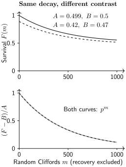
Calculated curves with the same $p=0.998$: $(A,B)=(0.499,0.5)$ and $(0.42,0.47)$. Both have normalized contrast $(F-B)/A=p^m$. The lower panel illustrates the model using known parameters; an experiment must estimate them with uncertainty.

A characteristic length is $m\sim1/(1-p)$ when $p$ is near one. Include short lengths, lengths across the decay, and sufficiently long lengths to constrain the offset. All points near the initial plateau cannot determine three parameters reliably.

Random sequences and repeated shots have different roles

At a fixed length, circuit $k$ has survival probability $q_k$. Execute $S$ independent shots on each of $K$ independently sampled circuits. Write

$$\begin{aligned} \sigma_{\rm seq}^2&=\operatorname{Var}(q_k),\\ v&=\mathbb E[q_k(1-q_k)]. \end{aligned}$$

The equal-weight mean of the observed circuit survival fractions obeys

$$\operatorname{Var}(\widehat F) =\frac{\sigma_{\rm seq}^2}{K}+\frac{v}{KS}.$$

The first term measures which circuits happened to be sampled; the second is conditional shot noise (Wallman and Flammia, 2014). Many repetitions of one circuit cannot replace independent circuit draws.

At a fixed total number of shots $N=KS$,

$$\operatorname{Var}(\widehat F) =\frac{S\sigma_{\rm seq}^2+v}{N}.$$

If new circuits have no extra cost, reducing $S$ cannot increase this variance. Large readout noise alone is not a reason to repeat fewer circuits. A practical reason is the overhead of generating, loading, or switching circuits. If that overhead is $c_s$ per circuit and a shot costs $c_h$, an interior continuous optimum is

$$S_{\rm opt}=\sqrt{\frac{v c_s}{\sigma_{\rm seq}^2 c_h}}.$$

Use at least one shot and account for integer counts and hardware limits. This is a design calculation under independent sampling, not a universal optimum for every RB experiment (Exercise 4).

For unequal shot counts, the equal-weight average of circuit fractions still targets the uniform circuit ensemble. Pooling all counts instead weights circuits by their shot counts; outcome-dependent allocation can then change the target.

Fit the original probabilities with an appropriate likelihood or weighted nonlinear regression. Taking $\log(\widehat F-B)$ can fail when the noisy difference is nonpositive and changes the noise model. Do not fix $B=1/d$ unless the measurement model justifies it.

For uncertainty, resampling whole circuit records within a length captures the variation of their observed means, including shot noise. Blindly adding a second resampling of their shots can count shot noise twice. A hierarchical parametric bootstrap is another option when the latent circuit-probability model is specified. Preserve circuit identity, counts, and acquisition time; Harper and colleagues (2019) discuss RB experimental design and inference.

Interleaving a target gate

Interleaved RB inserts a target Clifford $G_\star$ after every random reference Clifford and computes the inverse of the entire ideal product. Let the fitted rates be $p_{\rm ref}$ and $p_{\rm int}$.

For independent depolarizing reference and target errors,

$$\begin{aligned} p_{\rm int}&=p_{\rm ref}p_\star,\\ r_\star&=\frac{d-1}{d} \left(1-\frac{p_{\rm int}}{p_{\rm ref}}\right). \end{aligned}$$

For general errors this ratio is an estimate with systematic bounds, not a model-free fidelity identity (Magesan and colleagues, 2012). Reference and interleaved runs should be interwoven so drift is not confused with target error.

An exact coherent counterexample is instructive. Suppose every implementation is $U_\theta G$, where $U_\theta=e^{-i\theta Z/2}$, and interleave $X$. Since $XU_\theta=U_\theta^\dagger X$,

$$(U_\theta X)(U_\theta G)=XG.$$

The errors cancel within every interleaved pair. The remaining recovery error is a fixed edge contribution, so the interleaved curve has no interior decay: $p_{\rm int}=1$. Reference RB instead has

$$p_{\rm ref}=\frac{1+2\cos\theta}{3}<1.$$

The ratio would assign a negative target infidelity, although the target’s actual average infidelity is $(1-\cos\theta)/3>0$. Clipping that estimate to zero conceals the failure of the factorization assumption.

What one exponential cannot determine

The noise mechanism. A coherent $Z$ rotation and a stochastic $Z$ error can have the same RB decay. For the rotation,

$$r=\frac{1-\cos\theta}{3}, \qquad D_\diamond=|\sin(\theta/2)|,$$

where $D_\diamond$ is half the diamond norm distance. Small coherent errors have $r\sim\theta^2/6$ but $D_\diamond\sim|\theta|/2$. Hardware metrics develops these distinctions. Unitarity measurements add information about coherence, rather than converting one RB number into a universal guarantee (Wallman and colleagues, 2015).

Individual native-gate errors. If every Clifford contains exactly $L$ identical depolarizing native operations, then $p_{\rm C}=p_g^L$. Variable decompositions, different gates, idles, and coherent cancellations break that inference. Even a simplified random-length model averages $p_g^L$, not $p_g^{\mathbb E L}$.

A unique gate-by-gate fidelity. Gate dependence invalidates the elementary common-channel derivation. More general theory can justify a dominant exponential plus corrections under appropriate conditions (Wallman, 2018). Its relation to individually assigned gate errors depends on the gate-set representation (Proctor and colleagues, 2017). For example, implementing every Clifford as $WGW^\dagger$ still makes every ideal identity sequence return exactly, although gates can differ from their nominal matrices.

Closure of the computational space. Leakage and return from leaked levels add population dynamics. Measure total computational population as well as target survival; an unusual asymptote alone is not decisive because SPAM also changes $B$. A two-population leakage model is derived in Exercise 8 (Wood and Gambetta, 2018).

Stationarity or absence of memory. A mixture of rates can look nearly exponential over a short range. Randomize acquisition order, repeat reference lengths throughout the run, and inspect residuals and circuit distributions by time block. Length-dependent reset or readout can change the apparent rate. Noise with memory explains broader tests.

Question	Useful additional measurement
Does parallel activity change the error?	Compare isolated and simultaneous RB
Are errors coherent?	Unitarity or phase-sensitive sequences
Is population leaving the qubit space?	Leakage-resolving readout
How does a scheduled layer behave?	Cycle benchmarking
What channel acts on selected inputs?	Process tomography

These measurements address different questions. A precise RB fit is most useful when accompanied by its sampled gate set, compiler, timing context, and tested noise assumptions.

Exercises

1. The noisy recovery

For qubit depolarizing noise with parameter $p$ after every gate, including the inverse, derive the survival from $|0\rangle$. How do $A$ and $B$ change for an ideal inverse?

Solution

Depolarizing channels commute with unitary gates, and their parameters multiply. The ideal gates cancel, leaving $\mathcal D_{p^{m+1}}$. Thus $F=(1+p^{m+1})/2$, with $A=p/2$ and $B=1/2$. An ideal inverse removes one noise factor, so $A=1/2$. The exponent fitted against the number of random gates is still controlled by the same $p$.

2. A two-qubit error and its uncertainty

A fit gives $p=0.9920\pm0.0008$ as a one-standard-deviation statistical result. Convert to infidelity.

Solution

Here $d=4$, hence

$$\begin{aligned} r&=\tfrac34(1-p)=0.0060,\\ \sigma_r&=\tfrac34\sigma_p=0.0006. \end{aligned}$$

The result is $0.0060\pm0.0006$ under the RB model. This statistical uncertainty does not include model failure.

3. More circuits or more repetitions?

Take $\sigma_{\rm seq}^2=0.0004$ and $v=0.16$. Compare $(K,S)=(40,100)$ and $(100,40)$.

Solution

Both use 4,000 shots. Their variances are

$$\begin{aligned} V_1&=\frac{0.0004}{40}+\frac{0.16}{4000} =5.0\times10^{-5},\\ V_2&=\frac{0.0004}{100}+\frac{0.16}{4000} =4.4\times10^{-5}. \end{aligned}$$

More circuits reduce the first term. With no switching overhead, one shot on each of 4,000 circuits gives variance $(0.0004+0.16)/4000=4.01\times10^{-5}$. This compares total shots, not necessarily elapsed laboratory time.

4. Include switching time

For total time $T=K(c_s+Sc_h)$, derive $S_{\rm opt}$. Use the preceding variances with $c_s=10$, $c_h=1$ in common time units.

Solution

Eliminating $K$ gives

$$T\operatorname{Var}(\widehat F) =(\sigma_{\rm seq}^2+v/S)(c_s+Sc_h).$$

The terms depending on $S$ are $\sigma_{\rm seq}^2c_hS+vc_s/S$. Setting the derivative to zero gives the stated square root, about $63.25$ shots here. Compare feasible neighboring integers. If $c_s=0$, the optimum moves to the boundary $S=1$ when $\sigma_{\rm seq}^2>0$.

5. A depolarizing interleaved estimate

Let $p_{\rm ref}=0.9980$ and $p_{\rm int}=0.9940$ for one qubit. Calculate the ratio estimate. Is the same formula justified by a clean exponential alone?

Solution

$$\begin{aligned} p_\star&=0.9940/0.9980\simeq0.995992,\\ r_\star&=(1-p_\star)/2\simeq0.002004. \end{aligned}$$

No. The coherent cancellation example gives exact exponential behavior but violates scalar error factorization. Statistical fit precision and systematic validity are separate.

6. Equal RB decay, different errors

Compare $U_\theta$ with the channel $(1-q)\rho+qZ\rho Z$, taking $q=\sin^2(\theta/2)$. Show that their RB parameters agree and compare their half-diamond distances.

Solution

The coherent Bloch matrix has trace $1+2\cos\theta$. The stochastic Bloch matrix is $\operatorname{diag}(1-2q,1-2q,1)$, with the same trace. Both twirl to

$$p=\frac{1+2\cos\theta}{3}.$$

The distances are $|\sin(\theta/2)|$ for the rotation and $q=\sin^2(\theta/2)$ for the stochastic channel. At $\theta=0.02$, the common infidelity is approximately $6.67\times10^{-5}$, while the distances are approximately $0.01$ and $0.0001$.

7. A consistent change of frame

Every ideal Clifford $G$ is implemented perfectly as $WGW^\dagger$. What does an RB identity sequence do? For $G=X$ and $W=e^{-i\phi Z/2}$, calculate its nominal average infidelity.

Solution

Adjacent $W^\dagger W$ factors cancel, so the whole circuit is $WIW^\dagger=I$. RB sees no decay. Relative to nominal $X$, the error is a $Z$ rotation through angle $2\phi$, up to sign, giving

$$r_X=\frac{1-\cos(2\phi)}{3}.$$

A sequence-return experiment does not determine an absolute control frame. Relating its decay to nominal gate matrices needs a consistent choice of representation and complementary measurements.

8. Leakage and seepage

In a population model, a computational state leaks with probability $\ell$ per step, while a leaked state returns with probability $s$. Starting inside the computational space, derive its population $c_m$.

Solution

The recurrence is

$$c_{m+1}=(1-\ell)c_m+s(1-c_m).$$

For $\ell+s>0$,

$$c_m=\frac{s}{\ell+s} +\frac{\ell}{\ell+s}(1-\ell-s)^m.$$

For $\ell=0.02,s=0.01$, the limiting population is $1/3$ and the decay parameter is $0.97$. This is population exchange, not the qubit depolarizing parameter. Target-state survival also depends on how the remaining computational population is distributed.

9. Variable native-gate counts

Assume ideal recovery and independent random compilations using either one or three identical depolarizing native operations, equally likely for every Clifford. Find the effective parameter per Clifford and compare it with squaring $p_g$.

Solution

Each step averages independently, so

$$p_{\rm C}=\tfrac12(p_g+p_g^3).$$

The mean count is two, but

$$p_{\rm C}-p_g^2=\tfrac12p_g(1-p_g)^2.$$

Even this homogeneous model differs from using the mean exponent. The discrepancy is second order near $p_g=1$; real compilation-dependent errors need more information than a gate-count average.

References

• Harper, R., I. Hincks, C. Ferrie, S. T. Flammia, and J. J. Wallman. “Statistical analysis of randomized benchmarking.” Physical Review A 99, 052350 (2019). arXiv:1901.00535.
• Magesan, E., J. M. Gambetta, and J. Emerson. “Characterizing quantum gates via randomized benchmarking.” Physical Review A 85, 042311 (2012). arXiv:1109.6887.
• Magesan, E., and colleagues. “Efficient measurement of quantum gate error by interleaved randomized benchmarking.” Physical Review Letters 109, 080505 (2012). arXiv:1203.4550.
• Proctor, T., K. Rudinger, K. Young, M. Sarovar, and R. Blume-Kohout. “What randomized benchmarking actually measures.” Physical Review Letters 119, 130502 (2017). arXiv:1702.01853.
• Wallman, J. J. “Randomized benchmarking with gate-dependent noise.” Quantum 2, 47 (2018). arXiv:1703.09835.
• Wallman, J. J., and S. T. Flammia. “Randomized benchmarking with confidence.” New Journal of Physics 16, 103032 (2014). arXiv:1404.6025.
• Wallman, J., C. Granade, R. Harper, and S. T. Flammia. “Estimating the coherence of noise.” New Journal of Physics 17, 113020 (2015). arXiv:1503.07865.
• Wood, C. J., and J. M. Gambetta. “Quantification and characterization of leakage errors.” Physical Review A 97, 032306 (2018). arXiv:1704.03081.