State Tomography

Quantum state tomography estimates a density operator from measurements on many systems prepared by the same procedure. For a qubit, measurements along three independent axes determine its Bloch vector. For a general system, the measurements must distinguish every state in the chosen model.

The reconstruction is conditional on the assumed Hilbert space and calibrated detectors. Finite counts introduce uncertainty; drift and detector errors can invalidate the model even when the fitted density matrix is positive.

Required background. Density operators supply positivity and trace normalization; POVMs supply the Born probabilities for a general detector. Helpful background. Singular-value decomposition explains inversion and conditioning, and Fisher information explains local uncertainty estimates.

Reconstructing a qubit from three measurements

Write the state in the computational basis as

$$\rho=\frac12 \begin{pmatrix} 1+r_z&r_x-ir_y\\ r_x+ir_y&1-r_z \end{pmatrix}, \qquad |\mathbf r|\leq1.$$

The components are the Pauli expectations $r_x=\langle X\rangle$, $r_y=\langle Y\rangle$, and $r_z=\langle Z\rangle$. A measurement of axis $j$ returns $+1$ or $-1$, with

$$p_j(+)=\frac{1+r_j}{2}, \qquad r_j=2p_j(+)-1.$$

Measure different copies along each axis. If $N_j$ trials give $n_j^+$ positive outcomes, linear inversion replaces $p_j(+)$ by the frequency $n_j^+/N_j$.

For $1{,}000$ shots on each axis, suppose the counts are

Axis	Positive outcomes	Estimated component
$X$	$730$	$0.46$
$Y$	$610$	$0.22$
$Z$	$845$	$0.69$

Then

$$\widehat\rho_{\mathrm{LI}}= \begin{pmatrix} 0.845&0.23-0.11i\\ 0.23+0.11i&0.155 \end{pmatrix}.$$

Here $|\widehat{\mathbf r}|^2=0.7361$. Its eigenvalues $(1\pm|\widehat{\mathbf r}|)/2$ are about $0.929$ and $0.071$, so this estimate is physical. Its plug-in purity is

$$\operatorname{Tr}(\widehat\rho_{\mathrm{LI}}^2) =\frac{1+0.7361}{2}=0.86805.$$

A physical estimate is still an estimate. For independent binary trials,

$$\operatorname{Var}(\widehat r_j)=\frac{1-r_j^2}{N_j}.$$

Replacing the unknown $r_j$ by $\widehat r_j$ gives approximate standard errors $0.028$, $0.031$, and $0.023$. These omit calibration uncertainty and drift. Near a deterministic outcome, the plug-in error can vanish even though finite data do not prove exact certainty; the confidence region below avoids that problem. Nonlinear quantities such as purity also have sampling bias, even when the Bloch-vector estimate is unbiased (Exercise 2).

Which measurements determine a state?

For setting $s$ and outcome $a$, a known POVM effect $E_{a|s}$ predicts

$$p(a|s,\rho)=\operatorname{Tr}(\rho E_{a|s}), \qquad \sum_aE_{a|s}=I.$$

A design is informationally complete if distinct allowed states cannot give the same collection of probabilities. Measuring only $Z$ leaves $r_x$ and $r_y$ undetermined: for example, $|+\rangle\langle+|$ and $I/2$ both give equal $Z$ outcomes.

For dimension $d$, choose Hermitian operators with

$$B_0=I/\sqrt d,\qquad \operatorname{Tr}(B_\mu B_\nu)=\delta_{\mu\nu}.$$

A trace-one Hermitian matrix has coordinates

$$\rho=\frac Id+\sum_{\mu=1}^{d^2-1}\theta_\mu B_\mu.$$

Consequently the probabilities have the affine form

$$\begin{aligned} \mathbf p&=\mathbf c+A\boldsymbol\theta,\\ c_{a|s}&=\operatorname{Tr}(E_{a|s})/d,\\ A_{a|s,\mu}&=\operatorname{Tr}(E_{a|s}B_\mu). \end{aligned}$$

For unrestricted states, informational completeness is equivalent to $\operatorname{rank}A=d^2-1$. A single POVM needs at least $d^2$ outcomes, because its normalized probabilities contain at most one fewer independent number than its outcome count. Having enough outcomes is necessary, but their effects must also span the required directions.

Rank alone does not guarantee accuracy. Linear inversion gives $\delta\boldsymbol\theta=A^+\delta\mathbf f$, so a small singular value amplifies noise. If two measurement axes are almost parallel, they distinguish the missing perpendicular component only weakly. Tight, symmetric designs distribute sensitivity more evenly (Scott, 2006); tetrahedral qubit tomography is an example in Exercise 4.

For randomly chosen settings with known probabilities $w_s>0$, the joint effects $F_{s,a}=w_sE_{a|s}$ form one POVM. A dual frame satisfies

$$X=\sum_{s,a}\operatorname{Tr}(F_{s,a}X)D_{s,a}.$$

Replacing the joint probabilities by $n_{s,a}/N$ gives an unbiased linear estimate. For a fixed allocation of shots to settings, use the actual allocation weights or conditional frequencies; do not insert unrelated nominal random-setting weights. Data-dependent selection requires its own sampling model.

Enforcing positivity changes the estimator

Frequency fluctuations can give $|\widehat{\mathbf r}_{\mathrm{LI}}|>1$, hence a negative eigenvalue. That does not describe a new kind of state. It means the observed frequencies do not correspond exactly to any state in the assumed model.

In the slice $r_y=0$, take $\widehat{\mathbf r}_{\mathrm{LI}}=(0.90,0,0.80)$. Its length is $\sqrt{1.45}$, with a negative eigenvalue about $-0.102$. The nearest point in the Bloch ball under ordinary Euclidean distance is the radial projection

$$\widehat{\mathbf r}_{\mathrm{proj}} =\frac{(0.90,0,0.80)}{\sqrt{1.45}} \approx(0.747,0,0.664).$$

If deviations in $r_x$ receive four times the weight of deviations in $r_z$, the nearest point instead becomes approximately $(0.819,0,0.574)$. Both estimates are physical; they solve different optimization problems.

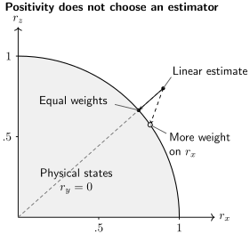
For $r_y=0$, physical states lie inside the unit disk. Radial projection minimizes equal-weight squared error. Giving the $x$ coordinate more weight moves the solution toward the measured $x$ value. Enforcing positivity does not select a unique statistical method.

Least squares and likelihood

A constrained least-squares estimate minimizes a quadratic residual over $\rho\succeq0$, $\operatorname{Tr}\rho=1$. With fixed positive weights this is convex. Multinomial frequencies within one setting are correlated, so a general weighted fit should use their covariance on the independent probability coordinates.

For independent repetitions of a stationary preparation, fixed setting counts $N_s$ give the log-likelihood

$$\ell(\rho)=\sum_{s,a}n_{a|s} \log\operatorname{Tr}(\rho E_{a|s}),$$

up to an irrelevant constant. Zero counts contribute zero; a positive count assigned zero probability gives log-likelihood $-\infty$.

Maximum likelihood maximizes $\ell$ over the state set. The log-likelihood is concave in $\rho$ (Exercise 5), so this is a convex optimization problem in the matrix variable. It is not generally a linear or unbiased estimator. A parameterization $\rho=TT^\dagger/\operatorname{Tr}(TT^\dagger)$ enforces positivity but makes the objective nonlinear in $T$. A generic semidefinite program with a linear objective is also different from this logarithmic likelihood problem.

For incomplete measurements, several states can maximize the likelihood. An additional maximum-entropy choice resolves that ambiguity by adding a criterion, not by extracting new measured information. Clipping negative eigenvalues and renormalizing is another possible rule, but it is generally neither maximum likelihood nor the closest state in a specified norm.

Bayesian estimation

With a specified prior measure, the posterior is proportional to likelihood times prior:

$$\pi(\rho|D)\propto\mathcal L(D|\rho)\pi(\rho).$$

The posterior mean is a physical density matrix. It minimizes posterior mean squared Hilbert–Schmidt error, but need not minimize a different loss. “Uniform over states” requires a measure, and priors can strongly affect small datasets or nearly pure states (Blume-Kohout, 2010).

No estimator is best for every reported quantity. The relevant choice depends on the sampling model and loss; positivity by itself does not guarantee an accurate fidelity or entanglement estimate (Schwemmer and colleagues, 2015).

A confidence region you can calculate

A point estimate says little about which nearby states remain plausible. For the three Pauli measurements, a simple finite-sample region follows from Hoeffding’s inequality for outcomes in $[-1,1]$:

$$\Pr\!\left(|\widehat r_j-r_j|>\delta_j\right) \leq2e^{-N_j\delta_j^2/2}.$$

Choose

$$\delta_j=\sqrt{\frac{2\log(6/\alpha)}{N_j}}.$$

A union bound then gives simultaneous coverage at least $1-\alpha$ for all three components. The region $C(D)$ contains the Bloch vectors satisfying

$$\begin{aligned} |\mathbf r|&\leq1,\\ |r_j-\widehat r_j|&\leq\delta_j \end{aligned}$$

for each $j=x,y,z$: the intersection of the three coordinate intervals with the Bloch ball.

For $N_j=1000$ and $\alpha=0.05$, $\delta_j\approx0.0979$. The region is deliberately conservative, but it is valid for every qubit state under the independent, calibrated measurement model, including pure states. It does not absorb unknown detector errors.

This guarantee concerns repeated datasets: at least 95% of regions produced by the procedure contain the fixed true state. A Bayesian 95% credible region instead contains 95% of posterior mass under its prior and likelihood. Tighter tomographic confidence regions can be constructed from binomial bounds (Wang, Scholz, and Renner, 2019).

For a derived quantity, minimize and maximize that quantity over $C(D)$. For example, the squared-fidelity convention for the target $|0\rangle$ gives $F_0=\langle0|\rho|0\rangle=(1+r_z)/2$. The worked data yield the conservative interval

$$F_0\in[0.796,0.894].$$

An empty intersection is possible: it signals data incompatible with the assumed model at this confidence level, although such an event can also occur through the allowed statistical failure probability.

For regular interior states, inverse Fisher information gives an asymptotic covariance estimate. Near the positivity boundary, Gaussian approximations and standard likelihood-ratio thresholds may fail. A bootstrap reruns the estimator on resampled data; its reliability depends on the model and resampling unit. It does not automatically repair boundary effects, calibration errors, or correlations.

What detector errors and drift can conceal

With symmetric binary readout flips of probability $\epsilon$,

$$m_{\mathrm{obs}}=(1-2\epsilon)r_z.$$

An observed contrast $0.6$ is consistent with $r_z=0.6,\epsilon=0$ or $r_z=1,\epsilon=0.2$. No amount of repeating this measurement separates the two unknowns. A calibrated $\epsilon\neq1/2$ permits inversion but amplifies statistical uncertainty. SPAM errors and measurement tomography explain the additional assumptions needed.

Drift also requires care. If every setting samples the same mixture of preparations, Born-rule linearity makes their average probabilities consistent with the same average state. For example, equal sampling of $|0\rangle$ and $|1\rangle$ in every setting reproduces $I/2$.

If different settings sample different preparations, there need not be one common average state. Preparing $|+\rangle$ during the $X$ block, $|+i\rangle$ during the $Y$ block, and $|0\rangle$ during the $Z$ block gives all three contrasts equal to one. Each block is physical, but combining them gives an impossible Bloch vector $(1,1,1)$. Interleave settings independently of the source, keep acquisition times, and compare repeated blocks (van Enk and Blume-Kohout, 2013).

Similarly, discarding outcomes can create setting-dependent accepted ensembles. Include losses in the measurement model unless the conditioning genuinely defines the same state before each setting choice. More shots shrink sampling error; they do not remove such bias.

Withheld or redundant measurements test whether a fitted state predicts new data. Residuals versus time and setting can reveal failures concealed by one average goodness-of-fit number. A positive matrix and small in-sample residuals alone cannot establish that detectors, preparation, and Hilbert-space truncation are correct.

Many qubits and narrower questions

For $n$ qubits,

$$\begin{aligned} \rho&=\frac1{2^n}\sum_{P\in\{I,X,Y,Z\}^{\otimes n}}r_PP,\\ r_P&=\operatorname{Tr}(\rho P). \end{aligned}$$

Normalization fixes the all-identity coefficient. There are $4^n-1$ remaining real parameters. Standard local Pauli tomography uses $3^n$ basis settings, each with $2^n$ possible bit strings. One setting estimates several commuting Pauli products from the same outcomes, with correlated errors.

Resource for eight qubits	Amount
Unrestricted state parameters	$65{,}535$
Local Pauli basis settings	$6{,}561$
Shots at $1{,}000$ per setting	$6{,}561{,}000$

Settings, outcomes, copies, and classical processing are different costs. Low rank and collective measurements can reduce copy requirements: Haah and colleagues (2016) give a theoretical bound of order $dr\log(d/\varepsilon)/\varepsilon^2$ for trace-distance error $\varepsilon$ and rank at most $r$. This assumes a measurement scheme acting collectively on copies; it is not the cost of ordinary local Pauli acquisition.

Structured reconstruction can exploit a justified low-rank or tensor-network model. If the question is only $\langle Z_1Z_2\rangle$, one $Z$ setting already suffices. Classical shadows estimate many selected properties; process tomography reconstructs transformations. Neither should be confused with a uniformly accurate full density matrix.

Exercises

1. Count independent directions

Why does an arbitrary $d$-dimensional state have $d^2-1$ real parameters, and why are $d^2$ outcomes necessary for one informationally complete POVM?

Solution

A Hermitian matrix has $d$ real diagonal entries and $d(d-1)/2$ complex off-diagonal entries, hence $d^2$ real parameters. Trace one removes one. Positivity bounds the region but does not reduce its interior dimension. An $m$-outcome normalized distribution has at most $m-1$ independent probabilities, so $m\geq d^2$ is necessary. Linear independence of the measurement directions is still required.

2. Purity has a bias even without positivity constraints

For independent Pauli measurements with $N_j>1$, show that $(1+\sum_j\widehat r_j^2)/2$ overestimates purity on average. Construct an unbiased scalar estimate.

Solution

Since $\mathbb E\widehat r_j=r_j$,

$$\mathbb E\widehat r_j^2 =r_j^2+\frac{1-r_j^2}{N_j}.$$

Thus the purity bias is $\tfrac12\sum_j(1-r_j^2)/N_j$. An unbiased estimate of $r_j^2$ is

$$q_j=\frac{N_j\widehat r_j^2-1}{N_j-1}.$$

Therefore $\widehat P_{\mathrm{unb}}=(1+\sum_jq_j)/2$ is unbiased and equals about $0.86692$ for the worked counts. It need not lie within the physical purity interval for every finite sample. Constraining a scalar estimate to that interval changes its bias.

3. Why weighting changes the projected state

In the $r_y=0$ slice, minimize $4(x-0.9)^2+(z-0.8)^2$ subject to $x^2+z^2\leq1$. Compare with radial projection.

Solution

The unconstrained minimum lies outside the disk, so the constraint is active. A Lagrange multiplier $\lambda>0$ gives

$$x=\frac{3.6}{4+\lambda}, \qquad z=\frac{0.8}{1+\lambda}.$$

Imposing $x^2+z^2=1$ gives $\lambda\approx0.39477$, hence $(x,z)\approx(0.81916,0.57357)$. Radial projection gives $(0.74741,0.66436)$. The weighted fit stays closer to the measured $x$ coordinate because moving it incurs a larger cost. Neither construction is automatically the binomial maximum-likelihood estimate.

4. Tetrahedral qubit tomography

Four unit vectors obey $\sum_k\mathbf n_k=0$ and $\mathbf n_j\cdot\mathbf n_k=-1/3$ for $j\neq k$. Show that $E_k=(I+\mathbf n_k\cdot\boldsymbol\sigma)/4$ is an informationally complete POVM.

Solution

Each effect has eigenvalues $1/2,0$, and the effects sum to $I$. Their probabilities satisfy

$$p_k=\frac{1+\mathbf n_k\cdot\mathbf r}{4}.$$

The tetrahedral vectors span three dimensions and obey $\sum_k\mathbf n_k\mathbf n_k^{\mathsf T}=(4/3)I_3$. Consequently

$$3\sum_kp_k\mathbf n_k=\mathbf r.$$

All three Bloch coordinates are determined.

5. Concavity of likelihood

For a trace-zero Hermitian direction $\Delta$, compute the second derivative of $\ell(\rho+t\Delta)$ where every positive-count event has positive probability.

Solution

Writing $p_{a|s}(t)=\operatorname{Tr}[(\rho+t\Delta)E_{a|s}]$ gives

$$\frac{d^2\ell}{dt^2} =-\sum_{s,a}n_{a|s} \frac{[\operatorname{Tr}(\Delta E_{a|s})]^2} {p_{a|s}(t)^2} \leq0.$$

The objective is concave. Strict concavity can fail when positive-count effects do not constrain a direction, so informational completeness of the intended design does not by itself guarantee uniqueness for every observed dataset.

6. Readout correction

A known symmetric readout error has $\epsilon=0.20$. Find the corrected contrast and its variance when the measured contrast is $\widehat m=0.60$ from $N=100$ trials. Explain why a plug-in Gaussian interval can be misleading.

Solution

The corrected estimate is $\widehat r_z=0.60/(1-0.40)=1$. Using the observed contrast in the binomial variance gives

$$\begin{aligned} \widehat{\operatorname{Var}}(\widehat r_z) &=\frac{1-0.60^2}{100(0.60)^2}\\ &\approx0.01778. \end{aligned}$$

The approximate standard error is $0.133$. A symmetric interval around one extends outside the allowed state range; truncating that interval does not automatically preserve a desired coverage. Finite-sample probability intervals can instead be transformed through the calibrated measurement model and intersected with the state set. Unknown calibration error requires additional uncertainty treatment.

7. Alternation and setting order

A source alternates between $|0\rangle$ and $|1\rangle$. Under what sampling condition do aggregate probabilities equal those of $I/2$? Does tomography establish independence between shots?

Solution

Each setting must sample equal numbers of the two states (or equal fractions in the corresponding expectation). Then its average probabilities equal those of $(|0\rangle\langle0|+|1\rangle\langle1|)/2=I/2$. Merely balancing the total dataset across states is insufficient if a setting is synchronized with the alternation. The sequence remains correlated even when all one-shot marginals match $I/2$; timestamps and odd/even comparisons can expose this.

8. A direct correlator

For eight qubits, compare full Pauli tomography with $1{,}000$ shots devoted to $\langle Z_1Z_2\rangle$. Find a worst-case standard error for the latter.

Solution

Full acquisition at $1{,}000$ shots per setting uses $3^8\times1000=6{,}561{,}000$ shots. One $Z$-basis setting suffices for the correlator: multiply the outcomes of qubits 1 and 2 and ignore the other outcomes. The product is $\pm1$, so its sample mean has variance at most $1/1000$ and standard error at most $0.0316$. This answers a narrower question without reconstructing other coherences.

9. Simultaneous confidence and target fidelity

Derive the component half-width for the 95% region with $N_j=1000$, and use $\widehat r_z=0.69$ to bound $F_0$. Must the three axes’ failure events be independent?

Solution

Give each component failure probability at most $\alpha/3$. Solving $2e^{-N\delta^2/2}=\alpha/3$ yields

$$\delta=\sqrt{\frac{2\log120}{1000}} \approx0.09785.$$

The fidelity half-width is $\delta/2$ and its center is $(1+0.69)/2=0.845$, giving $[0.79607,0.89393]$. A union bound needs no independence between failure events. The individual Hoeffding bounds still require their stated shot-sampling assumptions.

References

• Blume-Kohout, R. “Optimal, reliable estimation of quantum states.” New Journal of Physics 12, 043034 (2010). doi:10.1088/1367-2630/12/4/043034.
• Haah, J., A. W. Harrow, Z. Ji, X. Wu, and N. Yu. “Sample-optimal tomography of quantum states.” Proceedings of the 48th Annual ACM Symposium on Theory of Computing, 913–925 (2016). doi:10.1145/2897518.2897585.
• Schwemmer, C., L. Knips, D. Richart, H. Weinfurter, T. Moroder, M. Kleinmann, and O. Gühne. “Systematic errors in current quantum state tomography tools.” Physical Review Letters 114, 080403 (2015). doi:10.1103/PhysRevLett.114.080403.
• Scott, A. J. “Tight informationally complete quantum measurements.” Journal of Physics A: Mathematical and General 39, 13507–13530 (2006). doi:10.1088/0305-4470/39/43/009.
• van Enk, S. J., and R. Blume-Kohout. “When quantum tomography goes wrong: drift of quantum sources and other errors.” New Journal of Physics 15, 025024 (2013). doi:10.1088/1367-2630/15/2/025024.
• Wang, J., V. B. Scholz, and R. Renner. “Confidence polytopes in quantum state tomography.” Physical Review Letters 122, 190401 (2019). doi:10.1103/PhysRevLett.122.190401.