Certification of Entanglement

An entanglement test asks whether measured correlations can be explained by separable preparations. A convincing answer needs both a physical measurement model and an uncertainty bound. Here we turn a Bell-pair experiment into a numerical certificate, then compare what changes when one or both measurement devices are untrusted. The conclusion concerns specified subsystems and preparations; it does not automatically certify every emitted pair or the success of a later protocol.

Required background. Entanglement witnesses gives the separable bound for a target state. Negativity and the PPT criterion explains partial-transpose tests. CHSH gives the local and quantum correlation bounds.

Helpful background. State tomography explains reconstruction and confidence regions. We use the pure-target fidelity convention $F_\psi=\langle\psi|\rho|\psi\rangle$, without a square root.

Certifying a Bell pair from three measurements

For two identified qubits, let $|\Phi^+\rangle=(|00\rangle+|11\rangle)/\sqrt2$. Its fidelity and witness are

$$\begin{aligned} F_{\Phi^+}&=\frac{1+\langle XX\rangle-\langle YY\rangle+\langle ZZ\rangle}{4},\\ W&=\frac12I-|\Phi^+\rangle\langle\Phi^+|. \end{aligned}$$

Here $XX=X\otimes X$, and similarly for $YY,ZZ$. Every separable two-qubit state has $F_{\Phi^+}\leq1/2$, so $\langle W\rangle<0$ detects entanglement. Gühne and Tóth review these witness bounds. This is a test near a particular target: a different Bell state can be entangled while having zero overlap with $\Phi^+$.

On each trial, choose a common axis $j\in\{X,Y,Z\}$ uniformly at random, independently of the source and its previous history. Both stations measure that axis and return outcomes $a,b\in\{-1,1\}$. Consider these illustrative counts:

Axis	Product $ab=+1$	Product $ab=-1$	Correlator
$X$	940	60	$0.88$
$Y$	90	910	$-0.82$
$Z$	950	50	$0.90$

There are $N=3000$ trials, with 1000 in each setting in this example. The estimated fidelity is $0.90$, and the estimated witness is $-0.40$. These numbers alone do not yet include statistical or calibration uncertainty.

A single bounded score

Define $s_X=s_Z=1$ and $s_Y=-1$. The score for trial $i$ is

$$Z_i=\frac{1-3s_jab}{4}\in\{-1/2,1\}.$$

Uniform random settings give $\mathbb E Z_i=\operatorname{Tr}(W\rho_i)$ for ideal measurements, even if the prepared state $\rho_i$ changes between trials. Averaging the scores above gives $\widehat w=-0.40$. Unequal realized setting counts require using the trial scores, rather than blindly assigning equal weight to three estimated correlators; their equivalence here follows from the balanced counts.

Suppose calibration analysis guarantees that the measured conditional mean differs from the ideal witness by at most $b_{\mathrm{sys}}$. Under the hypothesis that every prepared state is separable, it is therefore at least $-b_{\mathrm{sys}}$. A bounded-increment concentration bound gives the conservative rejection rule

$$\begin{aligned} \delta_\alpha&=\frac32\sqrt{\frac{\log(1/\alpha)}{2N}},\\ \widehat w+b_{\mathrm{sys}}+\delta_\alpha&<0. \end{aligned}$$

It controls false rejection at level $\alpha$ for a fixed trial count, provided the conditional bound and fresh-setting assumptions hold on every round. Independence of the prepared states is unnecessary. With $\alpha=0.01$ and $b_{\mathrm{sys}}=0.015$,

$$\begin{aligned} \delta_{0.01}&\approx0.04156,\\ \widehat w+b_{\mathrm{sys}}+\delta_{0.01}&\approx-0.34344. \end{aligned}$$

The result rejects an always-separable source under these assumptions. It does not assign a 99% posterior probability to entanglement. Dirkse and colleagues develop more refined rejection and average-witness estimation methods with correlated noise and imperfect settings. A claim about a stationary state, an average state or each individual preparation must use the corresponding inference theorem.

Calibration and drift have physical consequences

More shots reduce sampling uncertainty, but cannot remove an unknown measurement bias. For ideal correlators $O_j$ and actual observables $\widetilde O_j$, the ideal and measured mean witness values satisfy

$$|\widetilde w-w|\leq\frac14\sum_{j=X,Y,Z}\|\widetilde O_j-O_j\|_\infty.$$

One may use the right side as $b_{\mathrm{sys}}$. Setting bias, crosstalk and leakage may require additional terms or an enlarged measurement model.

Randomizing the settings prevents a simple drift error. If the source knows the setting in advance, it can emit a separable state with $XX=1$ in the $X$ block, $YY=-1$ in the $Y$ block and $ZZ=1$ in the $Z$ block. Combining those blocks would falsely suggest $F_{\Phi^+}=1$, although no single state supplied all three correlations. Likewise, choosing the most negative witness after inspecting many candidates needs held-out data or simultaneous inference.

How much of the apparatus is trusted?

Test	Trusted quantum measurements	Conclusion from a valid violation
A calibrated witness	Both stations	Entanglement for the specified systems
Steering from Alice to Bob	Bob only	Alice can steer Bob; hence entanglement
A Bell test	Neither station	Nonlocal correlations; hence entanglement within quantum theory

All three need a justified trial definition, outcome treatment and statistical analysis. Bell tests additionally rely on sufficiently independent setting choices and absence of communication during a trial. Device independence removes detailed calibration assumptions, not these causal requirements.

Three explicit tests on the same noisy family

Consider

$$\rho_v=v|\Phi^+\rangle\langle\Phi^+|+(1-v)I/4,$$

with $0\leq v\leq1$. Its correlators are $(v,-v,v)$. The fidelity witness detects it when $v>1/3$; for this family that is also its exact entanglement threshold, as the PPT criterion confirms.

For steering, let Alice announce a binary result $A_j$ and let Bob trust three orthogonal Pauli axes $B_j$. A local hidden-state model obeys

$$T_3=\frac13\sum_{j=1}^3\langle A_jB_j\rangle\leq\frac1{\sqrt3}.$$

To see the bound, Bob’s hidden qubit state has a Bloch vector $\boldsymbol r$ of length at most one. Alice’s three responses have magnitudes at most one, so their scalar product with $\boldsymbol r$ is at most $\sqrt3$ by Cauchy–Schwarz; averaging over hidden states preserves the bound. Relabeling Alice’s $Y$ result gives $T_3=v$ for $\rho_v$. This three-axis test therefore detects steering for $v>1/\sqrt3$. Saunders and colleagues explain how additional settings can improve steering tests.

For CHSH, define $E_{xy}=\langle A_xB_y\rangle$ and

$$S=E_{00}+E_{01}+E_{10}-E_{11}.$$

The local bound is $|S|\leq2$. Appropriate Pauli-plane settings give $S=2\sqrt2\,v$, the maximum for this family, so a CHSH violation requires $v>1/\sqrt2$.

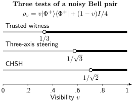
The same state can pass one test and fail another. Each solid segment marks strict detection above the open endpoint for the specified test. Only the first threshold is the entanglement boundary of this family; the steering and CHSH lines describe these particular measurement tests. Finite-data and systematic margins raise the visibility needed in practice.

At $v=0.60$, the trusted witness and this steering test detect entanglement, while CHSH does not. Failure of CHSH does not establish that every other Bell experiment is local, and failure of a chosen steering inequality does not establish the absence of steering.

Loss and postselection

Discarding no-click events can change the population being tested. Here is an explicit classical attack on a CHSH game with binary settings $x,y$ and outputs satisfying the winning condition $a\oplus b=xy$.

Before each trial, both stations share independent uniform guesses $x_*,y_*$. Alice reports only if $x=x_*$; Bob reports only if $y=y_*$. Alice outputs $a=0$ and Bob outputs $b=x_*y_*$. Whenever both report, they win. Coincidences occur with probability $1/4$, and the retained data have $S=4$, despite the entirely local construction. Each station merely uses its own setting and shared information.

A Bell test must include no-click outcomes, use an applicable loss-aware inequality, or use an event-ready herald chosen before the measurement settings. A trusted local quantum filter cannot create entanglement from a separable state, even conditionally. That physical statement does not justify arbitrary selection of recorded outcomes or correlations from incompatible subensembles. Bell experiments explains the detection and locality requirements.

What self-testing adds

A Bell violation certifies entanglement; self-testing asks whether it also identifies a target state up to unobservable local transformations and unused degrees of freedom. The review by Šupić and Bowles explains that equivalence. Robust statements need a theorem relating the measured score to a quantitative state bound.

Let $\Xi$ be the largest Bell-pair fidelity achievable by local trace-preserving extraction channels, without communication or postselection. Using squared fidelity as defined above, Kaniewski’s CHSH bound is

$$\begin{aligned} \Xi&\geq\max\{1/2,aS_{\mathrm{low}}+b\},\\ a&=\frac{4+5\sqrt2}{16},\qquad b=-\frac{1+2\sqrt2}{4}. \end{aligned}$$

Here $S_{\mathrm{low}}$ must be a valid lower bound for the correlations in the theorem. This particular bound improves on the trivial fidelity $1/2$ only above

$$S_* =\frac{16+14\sqrt2}{17}\approx2.10582.$$

At $S_{\mathrm{low}}=2.50$, it gives $\Xi\geq0.77275$. The straight line joining $(2,1/2)$ and $(2\sqrt2,1)$ is not a general lower bound; inserting it would overstate what CHSH alone certifies. The threshold $S_*$ describes this bound’s guarantee, not a separability boundary.

More parties and larger local spaces

The null set must match the question. For three or more parties, a biseparable state may mix preparations separable across different cuts. Excluding separability across each fixed cut separately need not exclude that mixture. Multipartite separability develops the distinction.

For a GHZ target, every biseparable state has fidelity at most $1/2$. Thus a valid lower bound above $1/2$ certifies genuine multipartite entanglement. One need not always measure the full projector: for independent commuting stabilizer generators $K_j$ with a unique common $+1$ state,

$$F_G\geq1-\frac12\sum_j(1-\langle K_j\rangle).$$

This follows because the probability of any failed stabilizer is at most the sum of its failure probabilities. It requires no statistical independence between generators. Tóth and Gühne develop efficient stabilizer-based entanglement tests. For GHZ states the fidelity threshold has the stated multipartite meaning; a different target needs its own biseparable bound.

Entanglement depth excludes mixtures of groups of at most $k$ parties, proving depth at least $k+1$. Genuine entanglement of all $N$ specified elementary parties corresponds to depth $N$. Bipartite Schmidt number instead concerns local dimension: fidelity to $|\Phi_d\rangle=d^{-1/2}\sum_j|jj\rangle$ exceeding $r/d$ excludes Schmidt number at most $r$. These are distinct questions about the same physical system.

For a small state, tomography may offer a broader search. In $2\times2$ and $2\times3$ dimensions, PPT is equivalent to separability; in larger dimensions it is only necessary. A negative partial-transpose eigenvalue of a noisy point estimate is insufficient by itself: the compatible confidence region must exclude the relevant null. Randomized shadow measurements can estimate many selected witnesses, with the calibration and simultaneous-inference assumptions still present. A measurement-device-independent witness shifts trust to supplied quantum input states; it should not be confused with a Bell test having only classical inputs.

Exercises

1. Reproduce the bounded score

Use the count table to find how often $Z=-1/2$ and $Z=1$, then calculate $\widehat w$. Why is the $Y$ sign reversed?

Solution

The target-sign events number $940+910+950=2800$, leaving 200 others. Hence

$$\widehat w=\frac{-2800/2+200}{3000}=-0.40.$$

The Bell state has $YY=-1$, unlike its $XX=ZZ=1$. Ignoring that sign estimates a different observable and can destroy the witness interpretation.

2. Bound an axis error

Suppose each implemented local binary observable differs from its ideal Pauli observable by operator norm at most $\eta=0.01$. Bound the correlator error and witness shift.

Solution

For norm-at-most-one observables,

$$\widetilde A\otimes\widetilde B-A\otimes B ={}(\widetilde A-A)\otimes\widetilde B +A\otimes(\widetilde B-B).$$

The triangle inequality gives an error at most $2\eta$ per correlator. The three coefficients each have magnitude $1/4$, so a sufficient witness margin is $3\eta/2=0.015$. This does not cover unmodeled leakage or crosstalk.

3. Is a negative mean enough to plan the experiment?

Suppose the expected witness is $-0.12$ and the systematic margin is $0.02$. At $\alpha=0.01$, how many trials make the expected value cross the conservative threshold? Does that guarantee a high probability of certification?

Solution

The available margin is $0.10$, so require

$$N>\frac{(3/2)^2\log100}{2(0.10)^2}\approx518.08.$$

Thus 519 trials place the mean beyond the threshold. They do not guarantee high power: the measured mean still fluctuates. Power planning must also bound those fluctuations under the proposed entangled source. If the systematic margin were at least $0.12$, increasing $N$ alone would never help.

4. Compare the noise thresholds

At $v=0.60$, calculate the Bell fidelity, three-axis steering score and optimal CHSH value. Which tests succeed before finite-data margins?

Solution

$$\begin{aligned} F_{\Phi^+}&=(1+3v)/4=0.70,\\ T_3&=0.60>1/\sqrt3,\\ S&=1.2\sqrt2\approx1.697<2. \end{aligned}$$

The witness and steering test succeed; CHSH does not. The three methods make different assumptions about the apparatus.

5. A local explanation of selected Bell data

Verify the joint detection probability and CHSH value in the guessing strategy above. Why does a herald before settings avoid this particular attack?

Solution

For every setting pair, both guesses match with probability $1/4$. On retained trials $a\oplus b=xy$, so $E_{00}=E_{01}=E_{10}=1$ and $E_{11}=-1$, giving $S=4$. A herald chosen before independent settings cannot select trials according to whether those later settings match the shared guesses. It must still satisfy the protocol’s other assumptions.

6. Use a valid self-testing bound

Evaluate the stated bound at $S_{\mathrm{low}}=2.05,2.50,2\sqrt2$. Why does the first case still certify entanglement?

Solution

The bounds are $1/2$, approximately $0.77275$, and $1$, respectively. At $2.05>2$, CHSH already rules out local models and hence separable states. This particular extractability inequality gives no improvement over the trivial $1/2$ there. Entanglement detection and a quantitative target-fidelity guarantee are different conclusions.

7. Stabilizers without independent errors

For a three-qubit GHZ target, measure $K_1=ZZI$, $K_2=IZZ$, $K_3=XXX$, each with a jointly valid lower bound $0.90$. What fidelity and entanglement conclusion follow?

Solution

Each stabilizer has failure probability at most $0.05$. The union bound gives $F_{\mathrm{GHZ}}\geq1-3(0.05)=0.85>1/2$, certifying genuine three-party entanglement. Multiplying three success probabilities would assume independence without justification. Simultaneous validity of the three lower bounds is needed.

8. Entangled across each cut but biseparable

Mix equally the three pure states

$$\begin{aligned} |\psi_A\rangle&=(|000\rangle+|011\rangle)/\sqrt2,\\ |\psi_B\rangle&=(|000\rangle+|101\rangle)/\sqrt2,\\ |\psi_C\rangle&=(|000\rangle+|110\rangle)/\sqrt2. \end{aligned}$$

Explain why the mixture is biseparable, although its partial transpose on each one-qubit subsystem has smallest eigenvalue $-\sqrt2/6$.

Solution

Each component is a product of one qubit in $|0\rangle$ and a Bell pair on the other two; the three terms use different cuts. Their mixture is therefore biseparable by definition. For the $A$ partial transpose, the subspace spanned by $|001\rangle,|010\rangle,|100\rangle$ contains

$$\frac16\begin{pmatrix}0&0&1\\0&0&1\\1&1&0\end{pmatrix},$$

with eigenvalues $0,\pm\sqrt2/6$. Permutation symmetry gives the same result for the other cuts. NPT across every fixed cut is therefore insufficient for genuine multipartite entanglement.

9. Dimension and selection

For $d=8$, a jointly valid fidelity lower bound is $0.64$. What Schmidt number follows? Would an uncorrected result selected from 200 candidate witnesses have the same confidence?

Solution

Since $5/8=0.625<0.64$, Schmidt number at most five is excluded, giving a lower bound of six. Since $6/8=0.75>0.64$, seven is not established. Searching 200 witnesses changes the statistical test; held-out confirmation or a simultaneous bound must include that selection.

10. A source that knows the next setting

Give separable states that produce the three ideal Bell correlators in separate, predictable setting blocks. Explain which assumption of the trial-score test fails.

Solution

Use $|+_x,+_x\rangle$ in the $X$ block, $|+_y,-_y\rangle$ in the $Y$ block and $|00\rangle$ in the $Z$ block. Every state is separable and produces the requested product deterministically. The setting is not independent of preparation. The score’s conditional expectation therefore need not equal the witness of a single prepared state, so the nonnegative separable bound cannot be applied.

References

• Dirkse, B., Pompili, M., Hanson, R., Walter, M., and Wehner, S. “Witnessing entanglement in experiments with correlated noise.” Quantum Science and Technology 5, 035007 (2020). doi:10.1088/2058-9565/ab8d88.
• Gühne, O., and Tóth, G. “Entanglement detection.” Physics Reports 474, 1–75 (2009). doi:10.1016/j.physrep.2009.02.004. The witness and separability results used here are reviewed in detail.
• Kaniewski, J. “Analytic and nearly optimal self-testing bounds for the Clauser–Horne–Shimony–Holt and Mermin inequalities.” Physical Review Letters 117, 070402 (2016). doi:10.1103/PhysRevLett.117.070402.
• Saunders, D. J., Jones, S. J., Wiseman, H. M., and Pryde, G. J. “Experimental EPR-steering using Bell-local states.” Nature Physics 6, 845–849 (2010). doi:10.1038/nphys1766.
• Šupić, I., and Bowles, J. “Self-testing of quantum systems: a review.” Quantum 4, 337 (2020). doi:10.22331/q-2020-09-30-337.
• Tóth, G., and Gühne, O. “Detecting genuine multipartite entanglement with two local measurements.” Physical Review Letters 94, 060501 (2005). doi:10.1103/PhysRevLett.94.060501.