Cross-Entropy Benchmarking

Cross-entropy benchmarking (XEB) asks whether a circuit’s measured bit strings tend to have high probability in the corresponding ideal circuit. The device supplies samples; a classical calculation supplies the ideal probability of each sampled string.

The commonly used linear XEB score is a correlation statistic. With suitable scrambling and noise assumptions it can estimate a circuit-fidelity parameter. By itself, it does not determine the full output distribution, quantum state fidelity, or computational advantage.

Required background. Why benchmarking is hard distinguishes a score from a physical claim; quantum circuit simulation explains the classical reference calculation. Helpful background. Relative entropy explains the logarithmic quantity from which XEB takes its name.

A score attached to each observed bit string

Let an $n$-qubit ideal circuit prepare $|\psi_U\rangle=U|0^n\rangle$, and set $D=2^n$. Its ideal probabilities are

$$p_U(x)=|\langle x|\psi_U\rangle|^2.$$

The device samples a distribution $q_U$. For each output $x$, assign the weight

$$Y_U(x)=Dp_U(x)-1.$$

Averaging $M$ observed weights estimates

$$\begin{aligned} X_U&=D\sum_xq_U(x)p_U(x)-1,\\ \widehat X_U&=\frac1M\sum_{i=1}^M Y_U(x_i). \end{aligned}$$

Linear XEB was used in the random-circuit experiment of Arute and colleagues (2019). It does not require estimating every probability of $q_U$.

For uniform sampling $u(x)=1/D$, the expected score is exactly zero for every normalized ideal distribution, regardless of scrambling. Ideal sampling instead gives

$$C_U=D\sum_xp_U(x)^2-1.$$

This ideal score is a shifted collision probability, not generally one. When $C_U>0$, define the circuit-normalized score

$$\widehat x_U=\frac{\widehat X_U}{C_U}.$$

With an exact fixed denominator, its expectation is one for ideal sampling and zero for uniform sampling. If the denominator is itself estimated, the ratio can be biased and its uncertainty must be propagated. Calling it “normalized” does not imply a model-free fidelity interpretation.

If $p_U$ is uniform, every weight vanishes and $C_U=0$. XEB then has no sensitivity to the sampler. Near-uniform circuits also have poor normalized sensitivity, as Exercise 7 quantifies.

A four-outcome calculation

Consider the ideal probabilities

$$p=(1/2,\ 1/4,\ 1/8,\ 1/8).$$

Mix ideal sampling with uniform sampling in proportions $0.6$ and $0.4$:

Outcome	Ideal $p$	Device $q$	Weight $4p-1$
$00$	$0.500$	$0.400$	$1$
$01$	$0.250$	$0.250$	$0$
$10$	$0.125$	$0.175$	$-1/2$
$11$	$0.125$	$0.175$	$-1/2$

The raw score is $0.400-0.175=0.225$. The ideal raw score is

$$C=4\left(\frac{11}{32}\right)-1=\frac38.$$

Therefore the normalized score is $0.225/0.375=0.6$, exactly the ideal-mixture weight. The total-variation distance between these distributions is instead $0.1$. The two numbers answer different questions.

Now change the device distribution to

$$q'=(1/2,\ 1/4,\ 1/4,\ 0).$$

Moving probability between the last two outcomes does not change the score, because they have equal weights. This device has the same XEB as ideal sampling despite a total-variation distance of $1/8$.

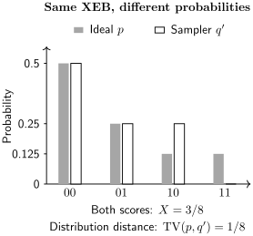
Different distributions, identical score. Probability moves between two outcomes with the same ideal probability, leaving $X=3/8$ and normalized XEB equal to one. The score cannot see this redistribution.

More generally,

$$X_U=D\langle q_U-u,\ p_U-u\rangle.$$

XEB measures one direction in a probability simplex with $D-1$ dimensions. Many changes in the output distribution are orthogonal to that direction.

Nor is the score bounded by one. Always returning the most likely output gives $X_U=Dp_{\max}-1$. In the example this is one, above the ideal raw value $3/8$, and its normalized score is $8/3$. A sampler can improve this score while becoming less faithful to the target distribution. Whether finding such outputs is computationally easy for a particular large circuit is a separate question.

What a depolarizing-mixture interpretation assumes

For the classical mixture

$$q_{U,f}=f p_U+(1-f)u, \qquad 0\leq f\leq1,$$

linearity gives $X_U=fC_U$. Hence normalized XEB estimates $f$ exactly under this distributional model.

A stronger quantum model is

$$\rho_{U,f} =f|\psi_U\rangle\langle\psi_U|+(1-f)\frac{I}{D}.$$

Its squared state fidelity with the pure target is

$$F_{\rm state}=f+\frac{1-f}{D}.$$

Even here the mixture weight differs from state fidelity at finite $D$. Observing the classical mixture does not establish the stronger quantum model: it specifies only the diagonal entries in the measurement basis.

For example, fully dephasing the ideal state preserves $p_U$ and its ideal XEB score, while its state fidelity becomes $\sum_xp_U(x)^2$. More strongly, the four-outcome distribution above can come from two orthogonal pure states, both with ideal XEB (Exercise 3). No measurement restricted to these probabilities can recover their relative phases.

For sufficiently scrambling circuits and specified weak-noise regimes, ensemble-averaged XEB can track a fidelity or no-error parameter. Errors near the output, spatially correlated errors, nonunital noise, and insufficient scrambling can invalidate the approximation. Gao and colleagues (2024) analyze these dependencies. An observed exponential in depth is not itself a proof of the noise model.

Why the ideal score is often close to one

For a Haar-random pure state in dimension $D\geq2$, a fixed output probability has density on $0\leq p\leq1$

$$h_D(p)=(D-1)(1-p)^{D-2}.$$

Its second moment is $2/[D(D+1)]$, so

$$\begin{aligned} \mathbb E_U\sum_xp_U(x)^2&=\frac2{D+1},\\ \mathbb E_U C_U&=\frac{D-1}{D+1}. \end{aligned}$$

For large $D$, the scaled probability $z=Dp$ approaches an exponential density $e^{-z}$. This is the Porter–Thomas approximation. It explains why an ideal raw XEB score is often described as one.

These are ensemble statements, not identities for a finite circuit. A shallow circuit, a structured circuit, or disconnected patches can have quite different collision probabilities. A random-looking histogram alone does not justify replacing $C_U$ by one.

There are also two ways to sample the probabilities. Choosing an output label uniformly gives the density $e^{-z}$; choosing it with its ideal Born probability gives the size-biased density $ze^{-z}$. Confusing them gives the wrong score moments.

For independent subsystems, the raw scores compose as

$$X_{12}+1=(X_1+1)(X_2+1).$$

The ideal collision normalizations obey the same shifted product law. Ordinary state fidelities of independent systems multiply without this shift. This difference matters when comparing a fully connected scrambling circuit with disconnected patches.

Statistical uncertainty for a fixed circuit

For independent shots on one fixed circuit,

$$\operatorname{Var}(\widehat X_U) =\frac{\operatorname{Var}_{q_U}(Y_U)}{M}.$$

An observed sample variance of the weights estimates the numerator. The normalized variance is divided by $C_U^2$ when $C_U$ is exact.

In the four-outcome mixture, $Y$ takes values $1,0,-1/2$ with probabilities $0.4,0.25,0.35$. Thus

$$\begin{aligned} \mathbb E Y&=0.225,\\ \mathbb E Y^2&=0.4875,\\ \operatorname{Var}(Y)&=0.436875. \end{aligned}$$

For $10{,}000$ independent shots, the raw standard error is approximately $0.00661$; the normalized standard error is $0.01763$. More shots shrink this sampling error, but do not remove a wrong reference model.

Under the large-$D$ Porter–Thomas mixture approximation,

$$\operatorname{Var}(Y)\simeq1+2f-f^2.$$

This is a planning approximation using the uniform and size-biased probability statistics, not a replacement for every fixed circuit’s variance. At small $f$, resolving a score with signal-to-noise ratio $z_\star$ requires roughly

$$M\gtrsim z_\star^2/f^2.$$

For $f=0.002$ and a nominal ratio of five, that is about $6.25$ million independent shots. Relative precision becomes costly as the score approaches zero.

Averaging circuits without changing the question

To estimate an equal-circuit ensemble average, first calculate each circuit’s score and then average those scores. Repeated shots on one circuit do not replace independent circuit instances.

Normalization and averaging do not generally commute. If circuit $k$ follows a mixture with weight $f_k$, then $X_k=f_kC_k$, and

$$\frac{\sum_k X_k}{\sum_k C_k} =\frac{\sum_k C_k f_k}{\sum_k C_k}.$$

This weights the mixture parameters by the circuits’ ideal contrast. It is not generally their equal-circuit mean. Pooling unequal numbers of shots adds another weighting by shot count. Exercise 6 gives a numerical example.

For $K$ independent circuits and $M$ shots per circuit, an equal-circuit raw-score mean has variance

$$\frac{\operatorname{Var}_U(X_U)}{K} +\frac{\mathbb E_U[\operatorname{Var}(Y_U\mid U)]}{KM}.$$

The first term is circuit variation; the second is shot noise. Time-correlated drift needs its own model or independently repeated blocks. Resample whole independent circuit or time-block records for a corresponding cluster analysis, or use a justified hierarchical model. Blindly resampling every level independently can double-count noise; treating all shots as independent circuit replicates can omit it.

When tuning gates with XEB, evaluate the final settings on fresh circuits. Interleave depths and circuit instances in time so a changing calibration is not confused with depth-dependent error.

Logarithmic cross-entropy difference

The earlier proposal by Boixo and colleagues (2018) used the logarithmic cross-entropy

$$H(q,p)=-\sum_xq(x)\log p(x),$$

with natural logarithms. Its difference from the uniform baseline is

$$\Delta H=H(u,p)-H(q,p).$$

Under $q=fp+(1-f)u$,

$$\Delta H=f[H(u,p)-H(p,p)].$$

Thus a nonzero exact ideal difference can normalize this statistic too. Under Porter–Thomas statistics, the ideal difference approaches one, but it is circuit dependent at finite size.

Linear XEB replaces the logarithmic weight with $Dp-1$ and is not itself an entropy. The logarithm is especially sensitive to tiny reference probabilities. If the ideal distribution has zeros, the uniform cross-entropy is infinite, so the baseline subtraction may be undefined; inserting a numerical floor changes the statistic.

The classical calculation and the stronger advantage claim

Every retained string needs an ideal reference probability. Computing selected probabilities can cost less memory than storing the full state, but can still take substantial time. Exact collision normalization may require more work than scoring observed strings. Circuit simulation and tensor networks explain the tradeoffs.

The reference must represent the implemented ideal circuit, including qubit ordering and measurement relabeling. If approximate probabilities are $\widetilde p=p+\delta p$, the population raw-score bias is

$$\Delta X=D\sum_xq(x)\delta p(x).$$

It obeys $|\Delta X|\leq D\|\delta p\|_\infty$. Normalization introduces additional sensitivity if $C$ is approximate. A simulator’s errors can average to zero under uniform output labels yet correlate with the device samples.

Acceptance rules also change the sampled distribution. Report acceptance alongside a conditional score. An unconditional score for rejected shots additionally requires a stated scoring rule or a model for their outcomes; multiplying a conditional score by acceptance is not a universal conversion.

XEB can diagnose hardware without establishing that a classical computer cannot attain the same score. Conditional hardness results depend on explicit circuit-family and computational assumptions (Aaronson and Gunn, 2020). Classical spoofing algorithms exist for particular families, including shallow circuits (Barak, Chou, and Gao, 2021). Gao and colleagues (2024) distinguish faithfully simulating dynamics from merely attaining a high score.

Use verification of quantum advantage for the separate comparison of classical algorithms, scores, and resources. Reduced or disconnected circuits can test a model for the target experiment, but their measured scores are not direct measurements of an unscored larger circuit.

Exercises

1. Endpoints and the mixture weight

Show that uniform sampling scores zero, ideal sampling scores $C$, and the normalized score of $q=fp+(1-f)u$ is $f$.

Solution

Normalization of $p$ gives $D\sum_xu(x)p(x)-1=0$. Substituting $q=p$ gives $C=D\sum_xp(x)^2-1$. By linearity, the mixture scores $fC$. Dividing by a nonzero exact $C$ gives $f$. When $p=u$, the statistic is identically zero and the division is undefined.

2. A high score from a poor sampler

Always return $00$ in the four-outcome example. Calculate raw XEB, normalized XEB, and total-variation distance from $p$.

Solution

The raw score is $4(1/2)-1=1$, and the normalized score is $1/(3/8)=8/3$. The total-variation distance is $1-p(00)=1/2$. The score exceeds the ideal value even though half the target probability mass is missing from the sampler.

3. Orthogonal states with identical XEB

Let $|\psi\rangle=\sum_x\sqrt{p_x}|x\rangle$ for the four-outcome example. Define $|\phi\rangle$ by leaving its $00$ amplitude positive and reversing the signs of the other three amplitudes. Find their state fidelity and XEB.

Solution

Both states have probabilities $p$. Their overlap is

$$\langle\psi|\phi\rangle =\frac12-\frac14-\frac18-\frac18=0.$$

The squared state fidelity is zero, but both give raw XEB $3/8$ and normalized XEB one. Computational-basis sampling cannot detect this phase change.

4. Derive the Porter–Thomas variance

For $Y=z-1$, use the densities $e^{-z}$ and $ze^{-z}$ to derive the mixture variance.

Solution

The exponential moments give $\mathbb E_u z=1$ and $\mathbb E_u z^2=2$, hence $\mathbb E_uY=0$ and $\mathbb E_uY^2=1$. Size bias gives $\mathbb E_p z=2$ and $\mathbb E_p z^2=6$, hence $\mathbb E_pY=1$ and $\mathbb E_pY^2=3$.

Mixing the two populations gives

$$\begin{aligned} \mathbb E Y&=f,\\ \mathbb E Y^2&=1+2f,\\ \operatorname{Var}(Y)&=1+2f-f^2. \end{aligned}$$

These moments use the large-dimension probability model. A fixed circuit with a different probability spectrum has different moments.

5. Finite-dimensional Haar normalization

Integrate $p^2$ against $h_D(p)$ to derive the ideal ensemble mean. What is it at $D=4$?

Solution

Using the beta integral,

$$\begin{aligned} \mathbb E p^2 &=(D-1)\frac{2!(D-2)!}{(D+1)!}\\ &=\frac2{D(D+1)}. \end{aligned}$$

Summing over $D$ outputs and inserting the factor $D$ in XEB gives $(D-1)/(D+1)$. At $D=4$ this is $3/5$, not one. The worked circuit’s $3/8$ is a particular realization, not the ensemble mean.

6. Normalize before or after averaging?

Two circuits have $(C_1,f_1)=(0.2,0.9)$ and $(C_2,f_2)=(1,0.3)$. Compare their equal-circuit normalized mean with the ratio of mean raw score to mean contrast.

Solution

The normalized mean is $(0.9+0.3)/2=0.6$. Their raw scores are $0.18$ and $0.30$, so

$$\frac{\overline X}{\overline C} =\frac{0.24}{0.60}=0.4.$$

The ratio places more weight on the high-contrast circuit. Neither averaging rule should silently substitute for the other.

7. Near-uniform targets

For a uniform device sampler and a nonuniform ideal distribution, show that $\operatorname{Var}_u(Y)=C$. Deduce the normalized standard error.

Solution

The mean is zero, and

$$\begin{aligned} \mathbb E_uY^2 &=\frac1D\sum_x(Dp_x-1)^2\\ &=D\sum_xp_x^2-1=C. \end{aligned}$$

Thus $\operatorname{Var}(\widehat x)=1/(MC)$ and the normalized standard error is $1/\sqrt{MC}$. As the target approaches uniformity, $C$ vanishes and the normalized estimator becomes less informative.

8. Accepted shots

A uniform sampler for the four-outcome example retains only output $00$. Find acceptance and conditional XEB. Why does multiplying the conditional raw score by acceptance fail to recover the original score?

Solution

Acceptance is $1/4$, and conditional raw XEB is one. The rejected outputs have weights $0,-1/2,-1/2$, with conditional mean $-1/3$. The unconditional score is

$$X=\frac14(1)+\frac34(-1/3)=0.$$

Using acceptance times conditional score would give $1/4$ because it implicitly assigns zero weight to rejection. That defines a different scoring rule.

9. Simulator bias and product systems

For the worked mixture, suppose the reference error is $\delta p=\eta(1,-1,0,0)$. Find the raw-score bias. Separately, what is the combined raw score of independent systems with scores $0.1$ and $0.2$?

Solution

For sufficiently small $\eta$, the reference remains a normalized distribution. Since $q_{00}=0.4$ and $q_{01}=0.25$,

$$\Delta X=4\eta(0.4-0.25)=0.6\eta.$$

Zero summed reference error does not imply zero score bias. For the independent systems, factorization gives $X_{12}+1=(1.1)(1.2)$, hence $X_{12}=0.32$. This is not the product $0.02$ of the two scores.

References

• Aaronson, S., and S. Gunn. “On the classical hardness of spoofing linear cross-entropy benchmarking.” Preprint, revised 2020. arXiv:1910.12085.
• Arute, F., and colleagues. “Quantum supremacy using a programmable superconducting processor.” Nature 574, 505–510 (2019). doi:10.1038/s41586-019-1666-5.
• Barak, B., C.-N. Chou, and X. Gao. “Spoofing linear cross-entropy benchmarking in shallow quantum circuits.” 12th Innovations in Theoretical Computer Science Conference, LIPIcs 185, 30:1–30:20 (2021). doi:10.4230/LIPIcs.ITCS.2021.30.
• Boixo, S., and colleagues. “Characterizing quantum supremacy in near-term devices.” Nature Physics 14, 595–600 (2018). arXiv:1608.00263.
• Gao, X., M. Kalinowski, C.-N. Chou, M. D. Lukin, B. Barak, and S. Choi. “Limitations of linear cross-entropy as a measure for quantum advantage.” PRX Quantum 5, 010334 (2024). arXiv:2112.01657.