Quantum Circuit Simulation

A classical circuit simulator computes properties of a quantum circuit: amplitudes, probabilities, observables or measurement samples. Storing the whole state is a useful general method, but it is often much more work than the question requires. The circuit’s structure and requested output determine which representation is useful.

The state and measurement rules follow the textbook treatment of Nielsen and Chuang. Here we develop local state-vector updates, measurement sampling and their cost. Specialized methods are introduced briefly and linked below. This differs from quantum simulation, where a controllable quantum system emulates another physical system.

Helpful background. Circuit Model defines gates and measurements. Tensor Product Ordering explains basis conventions, and Circuit Intermediate Representations explains quantum operations and classical conditions in a program.

Amplitudes, probabilities and samples

First decide which quantity to compute. Let $C$ be a circuit with unitary part $U_C$, input $\lvert\psi_0\rangle$, and a declared measurement. Common tasks include:

Task	Requested object	Typical use
full-state evolution	every amplitude of $U_C\lvert\psi_0\rangle$	debugging, small-system reference calculations
amplitude query	$\langle x\rvert U_C\lvert\psi_0\rangle$ for selected $x$	verification and path or tensor contractions
probability or marginal	$p(x)$ or $p(x_S)$	likelihoods, validation, conditional sampling
expectation value	$\langle O\rangle$	variational algorithms and observable prediction
weak sampling	bitstrings distributed according to the circuit	emulating terminal measurements
reduced state	$\rho_S$ for a small subsystem $S$	entanglement and local diagnostics
dynamic trajectory	outcomes and conditional state along one branch	feedforward, reset, and error-correction logic
channel or process	action on an operator basis or Choi representation	tiny-system verification of nonunitary behavior

The terms strong simulation and weak simulation are useful but have several precision conventions in the literature. Strong simulation generally means computing amplitudes, probabilities, marginals, or expectation values to a declared accuracy. Weak simulation means producing samples from the output distribution, exactly or within a declared distributional error. A full state vector is more information than either task normally requests.

The requested accuracy is part of the task. Exact algebraic output, floating- point state evolution, additive-error probabilities, relative-error rare-event probabilities, total-variation-accurate samples, and samples from a deliberately noisy model are different accuracy requirements.

Local state-vector updates

For an $n$-qubit pure state in the computational basis,

$$\lvert\psi\rangle = \sum_{x\in\{0,1\}^n} \psi_x\lvert x\rangle, \qquad \sum_x |\psi_x|^2=1.$$

An exact state-vector simulator stores the $2^n$ complex amplitudes $\psi_x$ to its chosen floating-point precision and applies each local gate directly to that array. “Exact” here means that no physical approximation or intentional truncation is made; ordinary finite-precision roundoff remains.

Index and bit-order convention

This page follows the register order of Circuit Model,

$$\lvert x_1x_2\cdots x_n\rangle = \lvert x_1\rangle_{Q_1} \otimes\cdots\otimes \lvert x_n\rangle_{Q_n},$$

and maps that bitstring to the integer

$$\operatorname{ind}(x) = \sum_{j=1}^{n} x_j2^{n-j}.$$

Thus $Q_1$ supplies the most significant displayed bit. Other libraries use other mappings. A simulator may reverse displayed strings, assign the lowest array-index bit to the top wire, or separate logical wire order from storage order. None of those choices is physically preferred, but every interface and test vector must declare the choice.

One-qubit update kernel

Let a one-qubit gate

$$G = \begin{pmatrix} g_{00} & g_{01}\\ g_{10} & g_{11} \end{pmatrix}$$

act on $Q_j$. Define the index offset $e_j=2^{n-j}$. For every basis index $x$ whose $j$th bit is zero, the simulator updates one disjoint amplitude pair:

$$\begin{pmatrix} \psi'_x\\ \psi'_{x+e_j} \end{pmatrix} = G \begin{pmatrix} \psi_x\\ \psi_{x+e_j} \end{pmatrix}.$$

Both old amplitudes must be read before either is overwritten. There are $2^{n-1}$ disjoint pairs, so each amplitude participates in exactly one update. A two-qubit gate similarly updates $2^{n-2}$ groups of four amplitudes, and a $k$-qubit gate updates $2^{n-k}$ groups of $2^k$ amplitudes. A dense matrix-vector multiplication within each group costs $O(4^k)$, so the total arithmetic is $O(2^{n+k})$. For fixed $k$, this is $O(2^n)$; structured diagonal or permutation gates can use cheaper kernels.

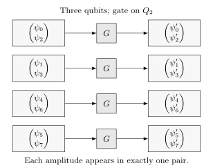
For three qubits, a gate on $Q_2$ couples indices separated by two. The four small updates can be computed independently; no $8\times8$ embedded matrix is needed. Subscripts denote integer array addresses.

Why local updates avoid a large matrix

The circuit unitary is a $2^n\times2^n$ matrix with $4^n$ complex entries. Constructing it explicitly throws away the main advantage of a local circuit description. If the goal is one output state, apply each local gate to a vector instead:

$$\lvert\psi_L\rangle = G_LG_{L-1}\cdots G_1 \lvert\psi_0\rangle.$$

For $L$ gates of bounded locality, a straightforward state-vector simulation uses

$$T=O(L2^n), \qquad M=O(2^n),$$

up to gate-specific constants and parallelization costs. The unitary itself needs $4^n$ complex entries; constructing it is useful only when the complete operation, rather than one output state, is requested.

A general channel is larger still. With $d=2^n$, a density matrix has $d^2=4^n$ entries, while a dense superoperator acts on those $d^2$ entries and has $d^4=16^n$ entries. A Choi matrix has the same dense size. Propagating one density matrix through local channels does not require storing the full channel. Structured or Kraus representations can reduce storage for particular channels.

State size and memory

With double-precision real and imaginary parts, one complex amplitude commonly occupies 16 bytes. The state array alone then requires

$$M_{\mathrm{sv}}(n) = 16\times2^n\ \mathrm{bytes}.$$

Qubits	State-vector storage
20	16 MiB
25	512 MiB
30	16 GiB
35	512 GiB
40	16 TiB
45	512 TiB

These are lower bounds for one state vector. Alignment, work buffers, fused gates, checkpoints, distributed halos or partner buffers, observables, and runtime overhead require additional memory. A machine advertised with 16 GiB cannot safely be assumed to simulate an arbitrary 30-qubit state in double precision.

Each added qubit doubles both state storage and the work of a generic local gate. Parallel hardware improves the constant and increases available memory; it does not remove the exponential scaling. Conversely, qubit count alone does not determine difficulty for specialized methods. A thousand-qubit Clifford circuit or a low-entanglement one-dimensional circuit may be easy for a structured representation, while a much narrower generic circuit may saturate state-vector memory.

A Bell state, step by step

Start in $\lvert00\rangle$, apply $H$ to $Q_1$, then a controlled-NOT with $Q_1$ as control and $Q_2$ as target. In basis order $\lvert00\rangle,\lvert01\rangle,\lvert10\rangle,\lvert11\rangle$, the initial state is

$$\boldsymbol\psi_0 = \begin{pmatrix} 1&0&0&0 \end{pmatrix}^{\mathsf T}.$$

The Hadamard acts on pairs separated by $e_1=2$:

$$\boldsymbol\psi_1 = \frac{1}{\sqrt2} \begin{pmatrix} 1&0&1&0 \end{pmatrix}^{\mathsf T}.$$

The controlled-NOT permutes the amplitudes associated with $\lvert10\rangle$ and $\lvert11\rangle$, giving

$$\boldsymbol\psi_2 = \frac{1}{\sqrt2} \begin{pmatrix} 1&0&0&1 \end{pmatrix}^{\mathsf T}.$$

A terminal computational-basis measurement returns 00 and 11 with probability $1/2$ each. Applying $X$ to either qubit changes these to 01 and 10, so the latter outcomes indicate different physics, not simply a reversal of the printed bit order.

The Bell state is symmetric under exchanging its two qubits. It therefore cannot test every ordering convention. Add an asymmetric check: applying $X$ to $Q_1$ in $|00\rangle$ must produce $|10\rangle$, stored at integer index two under our convention. A reversed control-target assignment also needs its own test: $H$ on $Q_1$ followed by CNOT with $Q_2$ as control leaves $(|00\rangle+|10\rangle)/\sqrt2$, rather than a Bell state.

Measurements and local observables

Terminal sampling

For a final computational-basis measurement, the ideal distribution is

$$p(x)=|\psi_x|^2.$$

After one state evolution, a simulator can construct a cumulative or hierarchical probability data structure and draw many terminal samples without reapplying the circuit. Sampling cost and preprocessing depend on the chosen data structure. The output order still has to be translated from storage bits to declared classical-register bits.

Finite shots estimate rather than reveal the distribution. For a Bernoulli event with empirical frequency $\widehat p$, Hoeffding’s inequality gives

$$\Pr\!\left( |\widehat p-p|\geq\epsilon \right) \leq 2e^{-2N\epsilon^2}.$$

Here the shots are independent draws from one fixed distribution. This sampling uncertainty is distinct from floating-point error and from any approximation made by the simulator.

Mid-circuit measurement

Suppose $Q_j$ is measured in the computational basis. The probability of outcome $m\in\{0,1\}$ is

$$p_m = \sum_{x:x_j=m} |\psi_x|^2.$$

For a sampled trajectory, draw $m$, zero amplitudes in the other branch, and renormalize:

$$\psi'_x = \begin{cases} \psi_x/\sqrt{p_m}, & x_j=m,\\ 0, & x_j\neq m. \end{cases}$$

This formula applies only to a sampled outcome with $p_m>0$; a zero-probability branch must never be normalized. The classical result must then be written to the declared classical register and may control later operations. A reset is not generally a unitary gate on the measured qubit; it can be implemented as measurement plus a conditional correction or as an explicit channel.

One trajectory produces one branch. Exact probabilities for all branches may require a branching tree whose width grows exponentially with the number of measurements. Repeating a dynamic circuit shot by shot can also require re-evolution after each branch point. Checkpointing, branch reuse, deferred measurement transformations, and classical-quantum state representations can reduce work in suitable circuits, but they must preserve the original outcome semantics.

Expectations and reduced states

If the requested output is an observable $O$, compute

$$\langle O\rangle = \langle\psi\rvert O\lvert\psi\rangle.$$

For a diagonal observable this is a weighted sum over $|\psi_x|^2$. For a Pauli string or other sparse local operator, apply a structured kernel and take an inner product. Constructing a dense $2^n\times2^n$ observable is normally as unnecessary as constructing the circuit unitary.

For a small subsystem $S$, the reduced state is

$$\rho_S = \operatorname{Tr}_{\bar S} \lvert\psi\rangle\langle\psi\rvert.$$

To compute this without building the full density matrix, regroup the amplitudes as a matrix $A_{ab}=\psi_{ab}$, where $a$ indexes the subsystem and $b$ its complement. Then

$$\begin{aligned} (\rho_S)_{aa'}&=\sum_b A_{ab}A^*_{a'b},\\ \rho_S&=AA^\dagger. \end{aligned}$$

The output has $4^{|S|}$ entries. Direct matrix multiplication costs $O(2^{n+|S|})$ arithmetic for a generic full state; with fixed small $|S|$ this is linear in the state-vector length. For the Bell state, $A=I/\sqrt2$ and $\rho_{Q_1}=I/2$: a pure global state can have a mixed local state. Partial Trace develops the subsystem algebra.

When circuit structure saves work

The best simulator depends on width, depth, gate structure, entanglement, non-Clifford resources, topology, requested output, and accuracy.

Method	Favorable circuit or output	Main cost
State vector	generic gates; many queries on one final state	$2^n$ amplitudes
Path sums and circuit cuts	few amplitudes; modest coupling across a cut	number of intermediate alternatives
Stabilizer methods	Clifford operations on stabilizer inputs	polynomial tableau updates
Tensor networks	favorable contraction graph or small required bond dimension	intermediate tensor size
Decision diagrams	repeated amplitude or operator structure	graph size, which can become exponential
Density matrix	a modest register with general mixed states or noise	$4^n$ entries
Stochastic trajectories	pure-state realizations of a noise model	state-vector cost times the number of trajectories

Stabilizer Simulation explains the algebraic compression of Clifford circuits, following Aaronson and Gottesman. Tensor-Network Simulation explains contractions and truncation; Markov and Shi relate simulation cost to the contraction graph. Noise Simulation compares density matrices with stochastic trajectories and their sampling error. An arbitrary non-stabilizer input does not become easy merely because all gates are Clifford.

State vector versus path summation

The state-vector, or Schrödinger, method propagates the whole wavefunction layer by layer. Runtime is approximately linear in circuit size for fixed width, but memory is exponential in width. It is attractive when many amplitudes, observables, or samples are needed from the same final state.

A path-sum, or Feynman, method expands selected outputs over intermediate indices. It can use much less memory, but the number of terms can grow exponentially with depth, cuts, or entangling gates. The method is attractive when only a few amplitudes are requested or when a circuit can be cut into weakly connected pieces. Hybrid algorithms trade state-vector width against the number of cut assignments.

Structure is a computational resource

Efficient classical simulation of a restricted circuit does not imply that all circuits of the same width are easy. Stabilizer methods exploit algebraic closure of Clifford operations. Tensor networks exploit a favorable contraction graph or bounded entanglement representation. Decision diagrams exploit repeated substructure. Low-depth geometry, few non-Clifford gates, limited Schmidt rank, commuting structure, or a small separator may each be useful, but they are different resources.

Accordingly, report more than qubit count. At minimum include gate counts by type, depth, connectivity, measurement placement, non-Clifford content, contraction or cut information for structured methods, and the requested output. Qubit count alone does not specify the computational difficulty.

Making state-vector updates faster

The calculation is often bandwidth bound

A generic local gate reads and writes nearly the entire state vector. For small gate matrices, data movement can dominate arithmetic. Performance therefore depends on contiguous access, cache reuse, vector instructions, memory channels, and avoiding unnecessary copies. A mathematically sparse one- or two-qubit gate does not make the evolved state sparse in general.

The target wire controls stride. Under this page’s indexing convention, a gate on $Q_n$ updates adjacent amplitudes, whereas a gate on $Q_1$ pairs amplitudes separated by half the array. Cache blocking or an internal qubit permutation can improve locality. If storage order changes, measurement strings and every later gate must use the same mapping.

Gate fusion

Gate fusion combines several nearby operations into one small dense kernel. It can reduce complete passes through memory and amortize dispatch overhead. Fusion is not free: a fused $k$-qubit matrix has $4^k$ entries and each local group contains $2^k$ amplitudes. Excessive fusion increases arithmetic, register pressure, compilation time, and cache demand.

A correct fusion pass must preserve dependency order, classical-control boundaries, measurement semantics, parameter values, and the declared floating-point contract. Comparing a fused simulator only with its own fused output is not independent validation.

Parallel and distributed updates

The disjoint amplitude groups of a local gate expose parallel work. CPUs can split groups across threads; GPUs can map them to many lanes; distributed systems can partition the state vector across ranks.

In distributed memory, some storage bits select the machine holding an amplitude; the remaining bits select its local address. A generic gate that mixes amplitudes across a machine-selecting bit needs data exchange or a layout change. A diagonal gate is an important exception: each amplitude is multiplied by a known phase, so it can be updated locally even when its target bit selects the machine. A permutation may sometimes be tracked by relabeling blocks.

Jones and colleagues describe distributed state-vector updates in QuEST; Fatima and Markov discuss memory access and related performance improvements. The communication cost depends on the gate as well as the target wire. An internal wire permutation must also be reflected in later gates and outputs.

Strong scaling eventually saturates when communication, synchronization, or fixed overhead dominates. Weak scaling can look excellent while total resources still double for every added generic qubit. Performance reports should include state precision, memory footprint, circuit family, gate mix, number of nodes or accelerators, communication volume, initialization and I/O policy, and whether compilation and sampling time are included.

Batched simulation

Parameter sweeps, gradients, noisy trajectories, and test suites may require many related state vectors. Batching can reuse gate metadata and improve accelerator occupancy, but it multiplies state storage. Shared prefixes can be checkpointed, provided later branches do not mutate the shared state. A batched throughput claim should state the number of states and latency per circuit; aggregate gates per second can conceal poor single-circuit latency.

Numerical errors and useful checks

Unitary evolution preserves norm mathematically, but floating-point kernels accumulate roundoff. Useful diagnostics include

$$\epsilon_{\mathrm{norm}} = \left| 1-\langle\psi\vert\psi\rangle \right|$$

and a round-trip error obtained by applying $U_C$ and then $U_C^\dagger$. Norm and inverse-circuit tests are necessary diagnostics but are not complete: a consistently wrong unitary can pass both. Compare small circuits with independently embedded gate matrices and asymmetric input states. Renormalizing after every gate can hide an unstable or nonunitary kernel; norm should be monitored before any corrective normalization.

Two state vectors that differ only by global phase represent the same pure state. A phase-insensitive comparison uses

$$F = \left| \langle\phi\vert\psi\rangle \right|^2, \qquad D = \sqrt{1-F}.$$

For normalized pure states, $D$ is their trace distance and bounds differences in measurement statistics. Elementwise array comparison without phase alignment can falsely reject an equivalent pure state. For a phase-sensitive amplitude query, however, retain the phase convention of the specified circuit. A gate phase also becomes relative phase when that gate is coherently controlled.

Single precision reduces memory and data traffic, sometimes substantially, but changes the error budget. Precision should be treated as a simulation parameter: compare against higher precision on representative circuits, track norm and conserved quantities, and test sensitivity as depth grows.

Approximate simulators introduce another error source. A mature result states whether the guarantee concerns state norm, fidelity, observable error, amplitude error, probability error, or total variation distance. A truncation tolerance internal to an algorithm is not automatically a bound on the reported physical quantity.

Dynamic circuits and reproducible comparisons

A dynamic simulation keeps the quantum state, classical measurement results and current program location. Measurement outcomes determine later branches; reset changes the state even if its measurement outcome is not retained. Discarding an entangled subsystem generally leaves a mixed state, so a pure state for the retained qubits alone may be insufficient.

Delay instructions affect the answer only through the chosen model: an ideal duration-independent gate model can omit idle evolution, whereas a model with dephasing or a drifting frame must evolve through the delay. A data-dependent loop can fail to terminate. A finite iteration cap is then a stopping rule; silently normalizing the completed trajectories changes the requested process. Circuit Intermediate Representations gives an explicit nontermination example.

For a reproducible comparison, state the input, gate definitions, basis and bit ordering, output quantity, precision and approximation settings. For samples, include the shot count and random-number settings. Compare numerical results with independently computed small examples; compare sample counts with their statistical uncertainty rather than demanding exact frequencies. Fixed seeds help reproduce a run, but one seed does not test a sampling distribution.

Report runtime and peak memory for the actual circuit and output task, including relevant setup, communication and sampling costs. A faster result on one circuit family need not be faster on another. An exponential generic state space does not rule out an efficient structured algorithm for a particular family.

Exercises

1. Derive the one-qubit pair update

For $n=3$ with basis order $\lvert000\rangle,\ldots,\lvert111\rangle$, list the amplitude pairs updated by a gate on $Q_2$.

Solution

Here $e_2=2^{3-2}=2$. Choose indices whose $Q_2$ bit is zero. The pairs are

$$(0,2),\quad(1,3),\quad(4,6),\quad(5,7).$$

In bitstrings they are

$$\begin{aligned} &(000,010),\quad(001,011),\\ &(100,110),\quad(101,111). \end{aligned}$$

Each pair is multiplied by the same $2\times2$ gate matrix, and the four pairs are disjoint.

2. Find a memory-limited qubit count

A node provides 256 GiB, but at least 25 percent must remain available for the runtime and work buffers. What is the largest double-complex state vector that fits under this policy?

Solution

The state may use at most $192$ GiB. A 33-qubit vector needs

$$16\times2^{33}\ \mathrm{bytes} = 128\ \mathrm{GiB},$$

while a 34-qubit vector needs $256$ GiB. Therefore the largest allowed vector has 33 qubits. This calculation does not guarantee good performance; it only checks the memory policy.

3. Compare vector and unitary storage

How much double-complex storage is required for a 15-qubit state vector and for the full 15-qubit unitary?

Solution

The state vector requires

$$16\times2^{15} = 524{,}288\ \mathrm{bytes} = 512\ \mathrm{KiB}.$$

The unitary requires

$$16\times4^{15} = 16\ \mathrm{GiB}.$$

The full matrix is $2^{15}=32{,}768$ times larger because it stores one output vector for every input basis vector.

4. Simulate a measurement collapse

The two-qubit state in basis order $00,01,10,11$ is

$$\lvert\psi\rangle = \frac{1}{\sqrt6} \left( \lvert00\rangle +\lvert01\rangle +2\lvert11\rangle \right).$$

Measure $Q_1$. Find both outcome probabilities and conditional states.

Solution

The $Q_1=0$ amplitudes have total probability

$$p_0 = \frac16+\frac16 = \frac13,$$

and the normalized state is

$$\lvert\psi_0\rangle = \frac{\lvert00\rangle+\lvert01\rangle}{\sqrt2}.$$

The $Q_1=1$ branch has probability $p_1=4/6=2/3$ and conditional state $\lvert\psi_1\rangle=\lvert11\rangle$.

5. Separate global phase from error

A reference state is $\lvert\phi\rangle$ and a simulator returns $\lvert\psi\rangle=-i\lvert\phi\rangle$. An elementwise difference is nonzero. What should a physical state comparison report?

Solution

The states differ only by global phase. Their overlap magnitude is one, so

$$F = |\langle\phi\vert\psi\rangle|^2 = 1, \qquad D=0.$$

A physical pure-state comparison should report agreement. If an application requires a phase relative to another coherent branch, that branch must be part of the simulated state rather than treated as an external global reference.

6. Distinguish strong and weak outputs

Backend A returns $p(0000)$ to additive error $10^{-8}$. Backend B returns bitstrings sampled from a distribution within total variation distance $10^{-3}$ of the target. Which is strong simulation and which is weak simulation?

Solution

Backend A performs a strong task because it estimates a specified output probability. Backend B performs a weak task because it samples from an approximately correct distribution. Neither contract automatically dominates the other: one accurate probability does not provide the full distribution, and sample access estimates rare probabilities inefficiently.

7. Identify distributed communication

A distributed state vector is partitioned so each rank owns contiguous blocks and the two most significant storage bits select the rank. Which one-qubit gates can be applied without exchanging amplitudes between ranks?

Solution

Gates on storage bits other than the two most significant bits pair amplitudes within each rank’s local block and need no inter-rank amplitude exchange. A generic mixing gate on either rank-selecting bit needs remote amplitudes or a layout change. A diagonal $Z$ or $R_z$ gate only multiplies local amplitudes by known phases and needs no amplitude exchange. A permutation may also admit virtual relabeling, depending on the implementation. Logical wire labels may be permuted onto storage bits, but that mapping must remain explicit.

8. A state, a unitary and a channel

At double-complex precision, compare the raw storage of one ten-qubit density matrix with that of a completely general dense ten-qubit superoperator.

Solution

The density matrix has $4^{10}=2^{20}$ entries and uses 16 MiB. The superoperator has $16^{10}=2^{40}$ entries and uses 16 TiB, a factor of $2^{20}$ larger. A ten-qubit unitary has the same raw size as the density matrix, not the general superoperator. Local Kraus updates can evolve a density matrix without constructing that enormous superoperator.

9. Explain why terminal sampling is cheaper

Why can one ideal state-vector evolution produce many terminal measurement shots, while a dynamic circuit with feedforward may require repeated evolution?

Solution

Terminal measurement does not affect any later quantum operation. Once the final probabilities $|\psi_x|^2$ are available, arbitrarily many classical samples can be drawn from that fixed distribution. In a dynamic circuit, a mid-circuit outcome collapses the state and selects later operations. Different shots can follow different quantum branches, so later evolution generally has to be performed for each sampled branch unless checkpoints or shared branch structure can be reused exactly.

10. Compute a reduced state without the full density matrix

For the state in exercise 4, form the coefficient matrix $A$ for $Q_1$ versus $Q_2$. Compute $\rho_{Q_1}$ and its purity. What changes if $Q_1$ is measured and its outcome ignored?

Solution

In the stated ordering,

$$\begin{aligned} A&=\frac1{\sqrt6}\begin{pmatrix}1&1\\0&2\end{pmatrix},\\ \rho_{Q_1}&=AA^\dagger =\frac16\begin{pmatrix}2&2\\2&4\end{pmatrix}. \end{aligned}$$

The purity is $\operatorname{Tr}(\rho_{Q_1}^2)=7/9$. Ignoring the outcome after a computational-basis measurement removes the off-diagonal entries, giving $\operatorname{diag}(1/3,2/3)$ with purity $5/9$. Taking a partial trace and performing an unread measurement are different physical operations.

References

• S. Aaronson and D. Gottesman, “Improved simulation of stabilizer circuits,” Physical Review A 70, 052328 (2004), doi:10.1103/PhysRevA.70.052328.
• A. Fatima and I. L. Markov, “Faster Schrödinger-style simulation of quantum circuits,” in 2021 IEEE International Symposium on High-Performance Computer Architecture, 194–207 (2021), arXiv:2008.00216.
• T. Jones, A. Brown, I. Bush, and S. C. Benjamin, “QuEST and high performance simulation of quantum computers,” Scientific Reports 9, 10736 (2019), doi:10.1038/s41598-019-47174-9.
• I. L. Markov and Y. Shi, “Simulating quantum computation by contracting tensor networks,” SIAM Journal on Computing 38, 963–981 (2008), doi:10.1137/050644756.
• M. A. Nielsen and I. L. Chuang, Quantum Computation and Quantum Information, 10th anniversary ed., Cambridge University Press (2010), doi:10.1017/CBO9780511976667.