Reproducing Quantum-Information Calculations

A reproducible notebook lets another reader reconstruct a calculation and understand why its answer should be trusted. Reversed qubit labels, an overlooked relative phase, or a mistaken sampling model can produce plausible output even when every cell runs.

This page develops a small example to paste into a Python notebook, then extends its checks to gates, channels, and algorithms. It does not provide a downloadable notebook. Existing downloads appear in the Notebook Index.

Helpful background. Quantum Circuit Simulation explains state vectors and measurement probabilities; Noise Simulation explains density matrices and trajectories. How to Use Computational Notebooks introduces the interface.

A two-qubit calculation with a known answer

Start with a question whose answer can be found independently of the code: does each probability refer to the intended qubit labels?

Write tensor factors as $|q_0q_1\rangle$, in the ordered basis $|00\rangle,|01\rangle,|10\rangle,|11\rangle$. The integer index is $k=2q_0+q_1$. This is our convention, not a universal software convention. Prepare

$$|\psi\rangle= \left(\frac{\sqrt3}{2}|0\rangle+ \frac12|1\rangle\right)\otimes|+\rangle,$$

where $|+\rangle=(|0\rangle+|1\rangle)/\sqrt2$. To prepare this state, start in $|00\rangle$ and apply $R_y(\pi/3)$ to $q_0$ and $R_y(\pi/2)$ to $q_1$, using

$$R_y(\theta)= \begin{pmatrix} \cos(\theta/2)&-\sin(\theta/2)\\ \sin(\theta/2)&\cos(\theta/2) \end{pmatrix}.$$

Multiplying the independent single-qubit probabilities gives

$$\begin{aligned} (p_{00},p_{01},p_{10},p_{11}) &=(3/8,3/8,1/8,1/8),\\ p(q_0=1)&=1/4,\\ p(q_1=1)&=1/2. \end{aligned}$$

This asymmetric state is a better ordering test than $(|00\rangle+|11\rangle)/\sqrt2$: exchanging the qubits leaves that Bell state unchanged. A test can pass because its input does not expose the error.

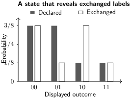
Filled bars use $|q_0q_1\rangle$; open bars exchange the labels. The probabilities of 01 and 10 change. Both distributions remain normalized, so normalization alone cannot reveal the mistake.

Calculate exact probabilities before drawing samples

This Python cell requires NumPy. It checks the matrix calculation against the analytic answer before sampling. The tolerance $10^{-14}$ is suitable for this tiny double-precision calculation, not a default for large systems.

import platform
import numpy as np

def ry(theta):
    c, s = np.cos(theta / 2), np.sin(theta / 2)
    return np.array([[c, -s], [s, c]])

zero = np.array([1.0, 0.0])
psi = np.kron(ry(np.pi / 3) @ zero,
              ry(np.pi / 2) @ zero)
p = np.abs(psi) ** 2
expected = np.array([3, 3, 1, 1]) / 8

assert abs(np.vdot(psi, psi) - 1) < 1e-14
np.testing.assert_allclose(
    p, expected, atol=1e-14, rtol=0
)

shots = 10_000
rng = np.random.Generator(np.random.PCG64(1729))
counts = rng.multinomial(shots, p)
q0_one = (counts[2] + counts[3]) / shots
sigma = np.sqrt(0.25 * 0.75 / shots)

print("Python:", platform.python_version())
print("NumPy:", np.__version__)
print("Order:", ["00", "01", "10", "11"])
print("Exact:", p)
print("Counts:", counts)
print("q0=1 estimate:", q0_one)
print("Model sampling SD:", sigma)

The exact result is fixed. The sampled estimate fluctuates around $0.25$, with standard deviation approximately $0.00433$ under independent repetitions. Do not assert that every sample must lie within one standard deviation: a correct sampler frequently falls outside that range.

Wrong exact probabilities suggest a state-preparation, gate-placement, or output-interpretation problem. Surprising samples with correct exact probabilities call for a statistical check.

Compare the intended physical objects

An array is meaningful only after its basis, units, and normalization are specified. When translating this example to a quantum SDK, prepare all four basis states and record how labels map to indices and displayed strings. Translate output back to the declared order before comparing it.

States and gates have different phase questions

For normalized pure states,

$$F=|\langle\psi_{\rm ref}|\psi\rangle|^2$$

ignores a common phase. Their density operators have trace distance $\sqrt{1-F}$. Test normalization first: otherwise the overlap need not define a fidelity in $[0,1]$. Computational-basis probabilities cannot test relative phase: $|+\rangle$ and $|-\rangle$ have identical $Z$ statistics and opposite $X$ outcomes.

For unitary matrices of dimension $d$, a useful comparison is

$$f_U=\frac{|\operatorname{Tr}(U^\dagger V)|}{d}.$$

After checking both matrices are unitary, $f_U=1$ means they differ by one common phase. Their controlled versions need not be equivalent: controlled-$I$ preserves a control in $|+\rangle$, whereas controlled-$(-I)$ changes it to $|-\rangle$. Controlled Operations explains why a formerly global phase becomes relative.

A channel must also work on entangled inputs

Checking traces of several outputs does not establish that a linear map is a quantum channel. Define the unnormalized Choi matrix with input first:

$$J=\sum_{i,j}|i\rangle\langle j| \otimes\mathcal E(|i\rangle\langle j|).$$

Complete positivity and trace preservation require

$$J\succeq0,\qquad \operatorname{Tr}_{\rm out}J=I_{\rm in}.$$

A normalized Choi matrix has trace one and output partial trace $I_{\rm in}/d$. Mixing conventions creates a factor-of-$d$ error.

Transposition preserves trace and sends every isolated density matrix to a positive density matrix, yet it is not completely positive: applying it to half of an entangled state can produce a negative eigenvalue. See Kraus, Choi, and Stinespring Representations.

Record residuals and negative eigenvalues before repairing matrices by normalization or projection. A repair changes the answer and can conceal a sign, ordering, or integration error. If roundoff is responsible, justify the tolerance using the calculation’s scale and conditioning.

Sampling, repeated tests, and uncertainty

A fixed seed helps investigate a particular run. It does not create more independent observations or eliminate uncertainty. Exact stream repetition can depend on the generator, sequence of calls, NumPy build, and environment; NumPy’s compatibility policy specifies these conditions.

For $K$ successes in $R$ independent trials with common probability $p$,

$$\widehat p=K/R,\qquad \operatorname{SD}(\widehat p)= \sqrt{\frac{p(1-p)}{R}}.$$

The standard deviation uses the true model probability. Substituting $\widehat p=0$ when no successes occur misleadingly gives zero estimated uncertainty.

For zero observed failures, the one-sided exact binomial upper confidence limit at confidence $1-\alpha$ follows from

$$(1-p_{\rm up})^R=\alpha,$$

and therefore

$$p_{\rm up}=1-\alpha^{1/R}.$$

At 95% confidence and $R=50\,000$, this is approximately $5.9913\times10^{-5}$, close to $3/R$. Confidence describes repeated-sampling coverage, not a posterior probability for the unknown rate. Correlated trials need a different analysis.

Twenty independent tests with false-alarm probability $0.05$ each have

$$P(\text{at least one false alarm}) =1-0.95^{20}\approx0.642.$$

Giving each of $m$ tests false-alarm probability at most $\alpha/m$ bounds the probability of any false alarm by $\alpha$, even without independence. This union-bound argument does not diagnose systematic bias.

Reuse of a calibration draw or environment can correlate trajectories. Follow the actual sampling hierarchy; Noise Simulation develops this point.

Make the calculation understandable from a fresh start

Arrange the notebook as an explanation: question and assumptions, parameters, reference prediction, numerical method, comparison, and interpretation. Rule and colleagues discuss how narrative structure helps readers follow executable work.

Restart the kernel and run cells from top to bottom. Otherwise a cell may use a variable left by a deleted or reordered cell. Also try a clean working directory with only declared files: a fresh kernel does not remove an old data file or cached result.

Record Python and package versions, an environment reconstruction file, input data and units, random generator and seeds, and the execution command. Save data behind plots. Sandve and colleagues explain why preserving inputs helps reconstruct numerical work; Environments gives practical guidance.

Jupyter’s NBClient executes notebooks in a selected working directory and by default stops on unexpected cell errors. Do not suppress ordinary errors with an option that continues past them. Expected exceptions in a teaching example should be tested explicitly. Execution checks whether code runs; physical comparisons test what it computes.

A cloud-device result also needs the circuit, returned counts, compilation settings, shot count, and relevant calibration time. A simulator rerun cannot reproduce the processor’s past noise. Preserve measured data and distinguish reanalysis from a new experimental run.

Choose a small calculation with a strong check

These suggested calculations have answers obtainable another way; they are not downloadable files.

Calculation	Independent comparison	What to vary
Grover search	Analytic success curve	Marked fraction and iterations, including overshoot
Teleportation	Corrected branches reproduce input	Complex input amplitudes and all four outcomes
Hamiltonian simulation	Small exact matrix exponential	Time step and noncommuting terms
VQE	Exact ground energy of the same Hamiltonian	Initializations, ansatz, and shots
Syndrome extraction	Hand-calculated Pauli syndromes	Correctable errors and measurement order

For Grover search from the uniform state, let $\sin^2\theta=M/N$, where $M$ of $N$ items are marked. After $r$ standard iterations,

$$P_r=\sin^2((2r+1)\theta).$$

Check an iteration curve, not just its maximum. For $N=8$, $M=1$, the first three probabilities are $1/8$, $25/32$, and $121/128$. More iterations eventually reduce success.

For VQE, an exact expectation of a Hermitian Hamiltonian in a normalized state satisfies $E\geq E_0$. A finite-shot estimator can fall below $E_0$ through sampling, and an error-mitigated estimator need not represent a positive state. Compare the same Hamiltonian and constants, report uncertainty, and include unsuccessful runs. The best of many starts answers a different question from the reliability of one new start.

For ideal teleportation with a shared Bell pair, averaging Bob’s state over Alice’s outcomes before he uses her message gives $I/2$. After correction using the message, each normalized branch reproduces the input. Nielsen and Chuang give the circuit identities underlying these comparisons.

Exercises

1. Detect exchanged labels

Exchange the example’s qubit labels while keeping the displayed basis order fixed. Find the distribution and total variation distance from the target.

Solution

The distribution becomes $(3/8,1/8,3/8,1/8)$. Only the middle entries differ, each by $1/4$, so

$$D_{\rm TV}=\tfrac12(1/4+1/4)=1/4.$$

Both distributions sum to one. Their $q_0=1$ probabilities are $1/4$ and $1/2$, making the marginal another useful test.

2. Find a phase that probabilities miss

A simulator returns $|-\rangle$ instead of $|+\rangle$. Compare their $Z$ probabilities and fidelity. Which measurement detects the problem?

Solution

Both $Z$ distributions are $(1/2,1/2)$, with total variation distance zero. The orthogonal states have $F=0$. Measuring $X$ gives $+1$ for the target and $-1$ for the returned state, each with certainty.

3. Check complete positivity

Show that the unnormalized Choi matrix of qubit transposition is SWAP, and find a negative eigenvalue.

Solution

Transposition sends $|i\rangle\langle j|$ to $|j\rangle\langle i|$, so

$$J_T=\sum_{i,j}|ij\rangle\langle ji|.$$

This exchanges the factors. The antisymmetric state $(|01\rangle-|10\rangle)/\sqrt2$ has eigenvalue $-1$; the three symmetric states have eigenvalue $+1$. The normalized Choi matrix has negative eigenvalue $-1/2$. The unnormalized output partial trace is still $I$.

4. Plan a rare-failure calculation

How many independent trials with zero failures are needed for a one-sided 95% upper confidence limit at most $10^{-4}$?

Solution

Require $1-0.05^{1/R}\leq10^{-4}$, or

$$R\geq\frac{\log(0.05)}{\log(1-10^{-4})}.$$

Rounding up gives $R=29\,956$. This describes what zero failures would establish; it does not guarantee observing zero failures. At very small rates use numerically stable functions such as log1p and expm1.

5. Choose a family error rate

You want 20 sampling tests to have probability at most $0.05$ of any false alarm. What per-test level suffices even for dependent tests?

Solution

Choose at most $0.05/20=0.0025$ per test. The probability of the union is at most the sum, $0.05$. Each test must itself satisfy its false-alarm guarantee under the assumed model.

6. Recognize an untested phase

A gate is tested on $|0\rangle$ and $|1\rangle$, measuring only $Z$ probabilities. Could both $I$ and $Z$ pass?

Solution

Yes: both preserve the basis probabilities. On $|+\rangle$, $I$ gives $|+\rangle$ whereas $Z$ gives $|-\rangle$. A superposition input and an $X$ measurement reveal the relative phase.

7. Interpret the best optimizer run

Twenty initializations produce one ground-state energy and nineteen much higher energies. Does the lowest value show that the optimizer usually succeeds?

Solution

It shows that the search found a good state once. Reliability concerns the distribution over the specified initialization procedure. Report all outcomes and the success criterion, including failed or terminated runs. The result depends on the problem instance and budget; it does not establish performance on other Hamiltonians.

8. Find hidden notebook state

A notebook fails after restarting its kernel. After that is fixed, it still fails in a clean folder. Give a likely cause for each failure.

Solution

The first may come from a variable defined in a deleted cell or cells run out of order. The second may come from an undeclared file or cached result. Put definitions in execution order and provide or generate every input. Saved outputs do not execute the code that originally produced them.

References

• M. A. Nielsen and I. L. Chuang, Quantum Computation and Quantum Information, 10th anniversary edition, Cambridge University Press (2010), doi:10.1017/CBO9780511976667 — states, channels, and algorithms.
• NumPy Developers, “Compatibility policy,” NumPy documentation, accessed 2026-10-15, official documentation — conditions for repeating pseudorandom streams.
• Project Jupyter, “Executing notebooks,” NBClient documentation, accessed 2026-10-15, official documentation — automated execution and errors.
• A. Rule et al., “Ten simple rules for writing and sharing computational analyses in Jupyter Notebooks,” PLOS Computational Biology 15, e1007007 (2019), doi:10.1371/journal.pcbi.1007007 — readable, executable explanations.
• G. K. Sandve, A. Nekrutenko, J. Taylor, and E. Hovig, “Ten simple rules for reproducible computational research,” PLOS Computational Biology 9, e1003285 (2013), doi:10.1371/journal.pcbi.1003285 — preserving computational inputs and context.