Calibration Loops

A calibration loop repeatedly measures a device, estimates how its parameters have changed, and adjusts the controls. For example, a Ramsey experiment can reveal a shifted qubit frequency; the next drive can then be retuned. The challenge is to follow real changes without mistaking measurement noise for drift or making a correction that harms another gate.

Calibration usually combines information from many experimental runs and changes later runs. This differs from a feedback pulse chosen from a measurement during one run, although the two can share hardware. We focus on estimation, update dynamics, interacting calibrations and independent checks of whether an adjustment helped.

Required background. Pulse-level control connects settings to gates; control and readout introduces calibration experiments; measurement as estimation explains uncertainty and likelihoods.

Measuring a frequency error

Suppose a qubit has angular-frequency detuning $\delta\omega$ from its drive reference. Choose the Ramsey analysis-phase convention so that the probability of one labeled outcome is

$$p(\delta\omega;t,\phi) =\frac{1+C(t)\cos(\delta\omega t+\phi)}2,$$

where $C(t)$ is the contrast and $\phi$ is a controllable phase. Independent shots at fixed settings give a binomial count; drift or memory between shots can invalidate that simple likelihood.

At $\phi=0$, positive and negative detuning give the same probability. Collecting more shots at that phase cannot distinguish their signs. Near zero detuning, choosing $\phi=\pi/2$ instead gives

$$p\simeq\frac12-\frac{C(t)t}{2}\,\delta\omega.$$

The signal now changes linearly with signed detuning. A longer wait increases phase sensitivity, but usually reduces contrast and narrows the unambiguous frequency range: at one fixed $t$, detunings separated by $2\pi/t$ have identical statistics at every analysis phase. Combine suitable waiting times or a sufficiently narrow prior range before using a local linear estimator. Rabi and Ramsey control develops the experiment; the point here is that choosing the measurements is part of the calibration, not a preliminary detail.

Why calibrations depend on one another

Calibration procedures are often bootstrapped. A readout classifier may depend on resonator frequency and amplifier state. A drive-amplitude calibration may depend on drive frequency, duration, transfer correction, and the classifier used to interpret outcomes. An entangling operation may depend on both single-qubit frames, coupler bias, neighbor state, and simultaneous-drive context.

Represent these dependencies by a directed graph $G_{\mathrm{cal}}=(V,E)$. An arrow $u\to v$ means that calibration $v$ uses setting $u$.

If a set $A\subseteq V$ changes, the conservative invalidation set is

$$\operatorname{Inv}(A) = A\cup\operatorname{Desc}_{G_{\mathrm{cal}}}(A).$$

Rechecking every dependent setting can be expensive. Record which upstream quantities matter and the range over which their variation was tested. If a readout frequency shifts within a tolerance already covered by a classifier’s robust validation region, the classifier need not automatically be refit. The earlier tests must actually cover the changed conditions.

Coupled parameters may need a joint fit

An acyclic dependency graph gives an order for the experiments. Physical parameters can nevertheless depend on one another in both directions: drive amplitude affects measured detuning, while the detuning estimate affects the amplitude fit. Treating that as an impossible graph is unhelpful. Instead, either:

1. group the coupled parameters into one calibration node;
2. define a fixed-point iteration with a convergence and stopping policy; or
3. break the cycle with a declared approximation and validate its residual.

The software dependency graph is also not the hardware resource graph. Two nodes can be logically independent yet unable to run concurrently because they share a readout line, laser, microwave source, cryogenic budget, or disturb one another through crosstalk.

Start a device from scratch with broader scans; maintain a working device with targeted checks near its current settings. These need different time and measurement budgets. Kelly and colleagues describe a practical dependency-graph approach.

Combining earlier estimates with new measurements

For an already localized frequency offset or gain, a scalar random-walk model is a useful starting point:

$$\theta_{k+1}=\theta_k+w_k, \qquad y_k=\theta_k+v_k.$$

Assume independent zero-mean process and measurement noise, with variances $Q$ and $R$, independent of the initial estimation error. The process noise describes change between measurements; the measurement noise describes uncertainty in each observation. Raw Ramsey counts are nonlinear observations; this model applies to a locally valid frequency estimate or a suitably linearized measurement, not automatically to the raw counts.

If the previous estimate has mean $m$ and variance $P$, predict the next mean as $m$ and variance as $P^-=P+Q$. On receiving $y$, update by

$$\begin{aligned} K&=\frac{P^-}{P^-+R},\\ m^+&=m+K(y-m),\\ P^+&=(1-K)P^-. \end{aligned}$$

A precise measurement has small $R$ and therefore receives more weight. A precise prior has small $P^-$ and changes less. With Gaussian initial uncertainty and Gaussian noises, these are exact Bayesian posterior moments. Under the corresponding second-moment assumptions without Gaussianity, the Kalman recursion gives the optimal linear estimate; a full nonlinear Bayesian estimate may differ. Kalman’s original paper develops the general vector formulation.

The covariance describes uncertainty within the chosen model. A wrong contrast, an aliased frequency, a sudden jump or a changed detector can make a very small reported variance misleading. Examine residuals and test the adjusted gate on independent data. Multimodal frequency estimates may require a distribution over several possible values rather than one mean and variance.

Drift can affect noise rates as well as control frequencies. Klimov and colleagues measured fluctuations in qubit relaxation times; a calibration model should track the quantities relevant to the operation being maintained.

Detecting drift without chasing noise

A monitor should detect operationally meaningful change without turning every statistical fluctuation into a parameter update. If a health measurement has prediction $\widehat y_k$ and innovation variance $S_k$, define the standardized innovation

$$z_k = \frac{y_k-\widehat y_k}{\sqrt{S_k}}.$$

A single threshold on $|z_k|$ catches abrupt excursions but is insensitive to small persistent shifts. A two-sided cumulative-sum monitor can use

$$\begin{aligned} C_k^+ &= \max\!\left(0,C_{k-1}^++z_k-\kappa\right), \\ C_k^- &= \max\!\left(0,C_{k-1}^--z_k-\kappa\right), \end{aligned}$$

and trigger when either statistic exceeds $h$. The allowance $\kappa$ sets the shift scale of interest; $h$ trades detection delay against false alarms. Correlated data, estimated baselines, and repeated monitoring alter the nominal false-alarm rate, so thresholds should be calibrated under the actual acquisition protocol.

For the scalar model above, the innovation is $y-m$ and its predicted variance is $S=P^-+R$. This includes both uncertainty in the predicted device state and measurement noise. Dividing only by $\sqrt R$ can produce too many alarms. The cumulative-sum method traces back to Page; Proctor and colleagues discuss time-resolved drift tests for quantum processors.

Repeated monitoring changes the meaning of a significance threshold. Even independent tests with a five-percent false-alarm probability each have probability $1-0.95^{20}\simeq0.642$ of at least one false alarm in twenty tests. Choose thresholds for a specified monitoring horizon or a sequential false-alarm criterion, and account for monitoring many devices. A correction for the number of qubits at one time does not by itself handle repeated looks over time.

A lower reset threshold than trigger threshold can prevent an alarm from rapidly switching on and off. More fundamentally, confirm that the monitor is connected, responsive and sensitive to the suspected drift. No alarm does not establish stability if the diagnostic has stopped working.

When several checks need attention, prioritize the likely effect on the upcoming computation together with the time and disturbance caused by recalibration. The oldest estimate is not necessarily the most consequential.

How strongly should a correction respond?

Calibration software can destabilize an otherwise usable device by applying updates too aggressively. Consider a fixed true parameter $\theta^\star$, an estimate $\widehat\theta_n$, and a noisy signed error observation

$$\begin{aligned} y_n&=\theta^\star-\widehat\theta_n+\varepsilon_n,\\ \mathbb E[\varepsilon_n]&=0,\\ \operatorname{Var}(\varepsilon_n)&=\sigma^2. \end{aligned}$$

For the proportional update

$$\widehat\theta_{n+1} = \widehat\theta_n+g\,y_n,$$

the estimation error $e_n=\theta^\star-\widehat\theta_n$ obeys

$$e_{n+1} = (1-g)e_n-g\varepsilon_n.$$

The noiseless loop is asymptotically stable exactly when

$$|1-g|<1, \qquad\text{or}\qquad 0<g<2.$$

For independent measurement noise and a stationary true parameter, the steady-state error variance is

$$\operatorname{Var}(e_\infty) = \frac{g}{2-g}\,\sigma^2.$$

For $0<g\leq1$, increasing gain removes a fixed offset faster; $g=1$ removes it in one noiseless update. For $1<g<2$, the error alternates sign, and its magnitude decays more slowly as $g$ approaches two. Thus larger gain does not always mean faster response. Small gain reduces injected measurement noise but follows real drift slowly. Dead bands, regularization, bounded steps, and model-based filtering are ways to shape this tradeoff. They do not replace a stability analysis.

To quantify the drift cost, let the true value change by an independent increment $w_n$ of variance $Q$ between updates, and write the measurement noise variance as $R=\sigma^2$. With the same timing convention,

$$e_{n+1}=(1-g)e_n+w_n-g\varepsilon_n.$$

The stationary variance before each measurement is

$$V(g)=\frac{Q+g^2R}{g(2-g)},\qquad 0<g<2.$$

It diverges as $g\to0$ when $Q>0$: averaging indefinitely cannot track a moving parameter. For $Q,R>0$, minimizing this variance gives

$$g_* =\frac{\sqrt{Q^2+4QR}-Q}{2R}.$$

This optimum lies between zero and one. It is a result for independent random-walk drift, direct measurements and instantaneous updates; delays, colored noise and nonlinear control response change it. In particular, the interval $0<g<2$ is not a universal rule for delayed feedback.

The same $g_*$ is the steady gain of the scalar Kalman filter above. At stationarity, its prediction and update obey $P^-=P^++Q$ and $P^+=RP^-/(P^-+R)$. Solving gives

$$P^-=\frac{Q+\sqrt{Q^2+4QR}}2=V(g_*), \qquad P^+=Rg_*.$$

The smaller $P^+$ is uncertainty immediately after the measurement. The curve below shows $P^-$ at the optimum: uncertainty before the next measurement, after another drift increment has added variance $Q$. For $Q/R=0.04$, these are $P^+/R\simeq0.1810$ and $P^-/R\simeq0.2210$. Comparing variances at the same time in the cycle therefore reconciles the two calculations.

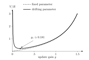
The dashed curve has a fixed true parameter; the solid curve includes random-walk drift with $Q/R=0.04$. Their vertical scale is variance divided by measurement-noise variance. The drifting case has its minimum at $g_*\simeq0.181$; very weak updates lag behind the changing parameter.

Designing measurements that identify the parameters

Choose experiment settings that distinguish the changes you need to detect. The Ramsey sign ambiguity is one example. A measured Rabi amplitude can also be confounded with readout contrast or imperfect preparation. Adding more shots to an indistinguishable model does not make it identifiable.

Randomizing or interleaving experimental settings can reduce bias from monotonic drift. Keep their acquisition order, and check whether reset memory, leakage or thermal transients correlate observations. Failed fits, multiple solutions and large residuals are information about the model or experiment, rather than reasons to return the last fitted value as a successful calibration.

How uncertainty affects dependent settings

If a derived parameter $y=f(\theta)$ depends smoothly on upstream estimates, first-order covariance propagation using the full joint covariance gives

$$\Sigma_y \approx J_f\Sigma_\theta J_f^{\mathsf T}, \qquad (J_f)_{ij} = \frac{\partial f_i}{\partial\theta_j}.$$

Shared data can correlate upstream estimates, so discarding off-diagonal covariances can overestimate or underestimate the derived uncertainty. This helps decide whether an upstream update matters for a dependent setting. However, first-order propagation is unreliable near nonlinear boundaries, discrete regime changes, or poorly identified directions. Replaying posterior samples or rerunning the descendant calibration may be safer.

Context must travel with uncertainty. A gate calibrated in isolation is not automatically valid during simultaneous operation. A readout classifier trained at one residual-excitation distribution is not automatically valid after a reset change. A transfer correction measured at one gain, temperature, or routing state may not extrapolate.

Error-Aware Compilation consumes these dated, context-qualified estimates. The compiler should not extend a calibration beyond its declared validity domain merely because no newer record exists.

Checking whether an adjustment helped

Use measurements not used for tuning to compare the old and new settings. Let $L_{\mathrm{cand}}$ and $L_{\mathrm{inc}}$ be losses measured on an interleaved held-out validation set, and define

$$\Delta = L_{\mathrm{cand}}-L_{\mathrm{inc}}.$$

For a required improvement margin $\delta>0$, one possible policy is

$$U_{1-\alpha}(\Delta)<-\delta,$$

where $U_{1-\alpha}$ is a one-sided upper confidence bound constructed for the sampling plan. Paired comparisons must include their covariance; correlated shots require an appropriate standard error. A maintenance update may instead use a noninferiority condition

$$U_{1-\alpha}(\Delta)<\delta_{\max},$$

combined with a reason to prefer the candidate, such as restored validity, lower drift sensitivity, or reduced resource cost.

Neither rule is sufficient by itself. Hard constraints may include leakage, worst-case or tail behavior, reset performance, readout assignment, thermal load, simultaneous-context error, and controller legality. The acceptance metric must match the operation’s use. Optimizing a single-qubit average score does not certify an entangling gate, a measurement instrument, or a logical cycle.

Choose the comparison metric, sample size or sequential stopping rule before inspecting its result. Repeatedly trying candidates against the same small test set can overfit that set, even if it was initially separate from the tuning data. A second diagnostic may expose a different failure, such as leakage hidden by an apparently improved average gate score.

Apply related parameter changes consistently. For example, a pulse tuned using a new frequency should not accidentally run with the old frequency. Keep enough information to reconstruct which settings were used for each batch, and check whether queued work still assumes earlier settings.

If the new settings fail, restoring earlier values can be useful, but it does not restore yesterday’s temperature, wiring or device frequency. Recheck the earlier settings in the current conditions. If neither set is usable, pause the affected experiments and diagnose the change rather than cycling through failed adjustments indefinitely.

Worked example: retuning a qubit

Consider five quantities for one transmon:

$$\begin{aligned} r&\longrightarrow c\longrightarrow a\longrightarrow g,\\ f&\longrightarrow a. \end{aligned}$$

Here $r$ is readout resonance, $c$ is the classifier, $f$ is drive frequency, $a$ is the $\pi/2$-pulse amplitude, and $g$ is a qualified single-qubit gate. The edge $c\to a$ records that the amplitude experiment used that classifier.

Ramsey measurements with a sign-sensitive analysis phase show a persistent frequency offset. A time-resolved fit estimates

$$\frac{\delta\omega}{2\pi} = (18\pm3)\,\mathrm{kHz}.$$

Here the quoted uncertainty is one standard error within the fitted model. The loop proposes a frequency correction and marks $a$ and $g$ stale. It does not invalidate $r$ or $c$ because the declared graph contains no path from $f$ to those nodes. If microwave leakage changes the readout response, that graph is incomplete and must be repaired.

After updating $f$, the loop reruns an error-amplifying amplitude experiment. Candidate and incumbent are then compared on interleaved independent batches under the same updated frequency, so the amplitude comparison does not mix two frequency settings. Let

$$\begin{aligned} \widehat\Delta&=-2.4\times10^{-4},\\ \operatorname{SE}(\widehat\Delta)&=0.6\times10^{-4}. \end{aligned}$$

Assume enough independent batches for a normal approximation and a preselected sample size. The one-sided $95\%$ upper bound is

$$\begin{aligned} U_{0.95}(\Delta) &= \widehat\Delta +1.645\,\operatorname{SE}(\widehat\Delta) \\ &\simeq -1.41\times10^{-4}. \end{aligned}$$

If the predeclared minimum improvement is $\delta=0.5\times10^{-4}$, then $U_{0.95}(\Delta)<-\delta$. Provided leakage, readout, and simultaneous-context hard limits also pass, the new amplitude is supported by this comparison.

The conclusion is narrow: the candidate improved the declared held-out loss under the measured context. It does not establish a universal gate fidelity, long-term stability, or application-level advantage. Keep the tested time window and settings with the result.

Exercises

1. Which measurements need repeating?

Consider the graph

$$\begin{aligned} r&\to c\to a\to g,\\ f&\to a. \end{aligned}$$

Which nodes are conservatively invalidated when $f$ changes? Give a valid recalibration order. Does $c$ need to run again?

Solution

The descendants of $f$ are $a$ and $g$, so

$$\operatorname{Inv}(\{f\}) = \{f,a,g\}.$$

After setting the new $f$, run $a$ and then $g$. Node $c$ is not a descendant of $f$, so the declared graph does not require it to rerun. If the physical frequency change can alter readout, the graph or its assumptions about the context is incomplete.

2. Correlated parameter errors

Two estimates have variances $s^2$ and covariance $c$. A derived setting is their difference. Find its variance for $c=0$, $c=s^2$ and $c=-s^2$.

Solution

For $y=\theta_1-\theta_2$, covariance propagation is exact because the function is linear:

$$\operatorname{Var}(y)=2s^2-2c.$$

The three answers are $2s^2$, zero and $4s^2$. Fully shared errors cancel in the difference; perfectly anticorrelated errors reinforce. These extreme cases are valid positive-semidefinite covariance matrices, although they are singular. Treating the estimates as independent would miss both limits.

3. Proportional-loop stability

For

$$\widehat\theta_{n+1} = \widehat\theta_n +g(\theta^\star-\widehat\theta_n+\varepsilon_n),$$

derive the noiseless stability interval and the steady-state variance for independent noise of variance $\sigma^2$.

Solution

With $e_n=\theta^\star-\widehat\theta_n$,

$$e_{n+1} = (1-g)e_n-g\varepsilon_n.$$

Noiseless convergence requires $|1-g|<1$, hence $0<g<2$. If the stationary variance is $V$,

$$V = (1-g)^2V+g^2\sigma^2.$$

Solving gives

$$V = \frac{g}{2-g}\,\sigma^2.$$

Increasing $g$ from zero to one speeds noiseless correction but increases measurement-noise variance. Increasing it from one toward two produces slower alternating decay as well as more noise.

4. A CUSUM trigger

Let $\kappa=0.5$, $h=2.5$, $C_0^+=0$, and standardized innovations be

$$0.4,\quad1.3,\quad1.5,\quad0.2,\quad1.8.$$

At which sample does the positive CUSUM first trigger?

Solution

The recurrence gives

$$\begin{array}{c|ccccc} k & 1 & 2 & 3 & 4 & 5\\ \hline C_k^+ & 0 & 0.8 & 1.8 & 1.5 & 2.8 \end{array}$$

The statistic first exceeds $h=2.5$ at sample 5. The result assumes the standardized innovations and threshold calibration are valid for this data stream.

5. Improvement is stronger than noninferiority

A fixed-size paired comparison estimates new minus old loss as $\widehat\Delta=-0.2\times10^{-4}$, with standard error $0.4\times10^{-4}$. Using the normal multiplier $1.645$, test both a required improvement of $0.5\times10^{-4}$ and an allowed worsening of at most $0.5\times10^{-4}$.

Solution

The one-sided upper bound is

$$\begin{aligned} U_{0.95}&=(-0.2+1.645\times0.4)10^{-4}\\ &=0.458\times10^{-4}. \end{aligned}$$

It is not below $-0.5\times10^{-4}$, so the improvement criterion fails. It is below $+0.5\times10^{-4}$, so the stated noninferiority criterion passes under the assumed sampling model. This does not establish equality or improvement. A lower time cost or more stable control might still make the new setting useful, provided the other required performance limits pass.

6. One scalar Kalman update

A frequency-offset prior has mean $12\,\mathrm{kHz}$ and variance $25\,\mathrm{kHz}^2$. A direct measurement gives $20\,\mathrm{kHz}$ with noise variance $9\,\mathrm{kHz}^2$. Assume the measurement matrix is one and no additional process noise is added. Find the posterior mean and variance.

Solution

The gain is

$$K = \frac{25}{25+9} = \frac{25}{34} \simeq 0.735.$$

Therefore

$$\begin{aligned} \widehat\theta_{\mathrm{post}} &= 12+\frac{25}{34}(20-12) \simeq 17.88\,\mathrm{kHz}, \\ P_{\mathrm{post}} &= \left(1-\frac{25}{34}\right)25 \simeq 6.62\,\mathrm{kHz}^2. \end{aligned}$$

The calculation is conditional on the linear Gaussian model.

7. Resource-constrained scheduling

Node $A$ calibrates readout resonance in 3 minutes on the readout resource. Node $B$ performs drive spectroscopy in 4 minutes on the drive resource. Node $C$ trains the classifier in 2 minutes on the readout resource and depends on $A$. Node $D$ calibrates pulse amplitude in 3 minutes on the drive resource and depends on both $B$ and $C$. Find the shortest schedule under these resource assumptions.

Solution

Run $A$ and $B$ in parallel from minute 0. Then:

• $A$ finishes at minute 3, so $C$ runs from 3 to 5;
• $B$ finishes at minute 4;
• $D$ waits for both parents and runs from 5 to 8.

The makespan is 8 minutes. A serial execution would take 12 minutes. This schedule is legal only if the readout and drive experiments are also experimentally compatible when concurrent.

8. Ramsey signs and frequency aliases

At one waiting time $t$, a calibration uses only $\phi=0$. Can it distinguish $\delta\omega$ from $-\delta\omega$? What changes if it also uses $\phi=\pi/2$? Does this resolve all frequency ambiguity?

Solution

The cosine is even, so the first experiment cannot distinguish the signs. The second measures $[1-C\sin(\delta\omega t)]/2$, which generally distinguishes them and gives linear sensitivity near zero. Together they identify phase modulo $2\pi$, not an unrestricted frequency. Offsets $\delta\omega+2\pi n/t$ remain indistinguishable for every integer $n$. Use prior localization or additional suitable waiting times to select the frequency branch. At special phases such as zero or $\pi$, the two signs already coincide modulo $2\pi$.

9. Restoring earlier settings after a temperature change

A candidate pulse fails validation after an abrupt refrigerator-temperature excursion. The previous pulse passed yesterday. Is restoring that pulse sufficient?

Solution

No. Rollback restores the previous control artifact but does not restore yesterday’s physical state. Recheck the earlier pulse at the new temperature and with the current related settings. If it also fails, suspend the affected measurements while diagnosing the change.

10. Optimize the gain for a drifting parameter

For independent random-walk drift with $Q/R=0.04$, minimize the variance $V(g)$ above. Compare $g=0.05$, $g=1$ and the optimum.

Solution

Differentiating gives the condition

$$Rg^2+Qg-Q=0.$$

The positive root is $g_*\simeq0.1810$. The normalized variances are

$$\begin{aligned} V(0.05)/R&\simeq0.4359,\\ V(1)/R&=1.04,\\ V(g_*)/R&\simeq0.2210. \end{aligned}$$

The weak update lags behind drift; replacing the estimate with each new measurement injects too much measurement noise. The intermediate gain balances them within the stated model. These are variances, so RMS errors are their square roots times $\sqrt R$.

References

• R. E. Kalman, “A new approach to linear filtering and prediction problems,” Journal of Basic Engineering 82, 35–45 (1960), doi:10.1115/1.3662552.
• J. Kelly, P. O’Malley, M. Neeley, H. Neven, and J. M. Martinis, “Physical qubit calibration on a directed acyclic graph” (2018), arXiv:1803.03226.
• P. V. Klimov et al., “Fluctuations of energy-relaxation times in superconducting qubits,” Physical Review Letters 121, 090502 (2018), doi:10.1103/PhysRevLett.121.090502.
• E. S. Page, “Continuous inspection schemes,” Biometrika 41, 100–115 (1954), doi:10.1093/biomet/41.1-2.100.
• T. Proctor, M. Revelle, E. Nielsen, K. Rudinger, D. Lobser, P. Maunz, R. Blume-Kohout, and K. Young, “Detecting and tracking drift in quantum information processors,” Nature Communications 11, 5396 (2020), doi:10.1038/s41467-020-19074-4.