Optimal Control for Quantum Processors

Quantum optimal control searches for a pulse or feedback rule that makes a physical system perform a chosen task. The first decision is what that task means: transferring one state, implementing a gate on every input, and resetting a noisy qubit are different objectives. A very successful search can still solve the wrong one.

This page explains how to choose a control representation and search method, then test the result on a quantum processor. The dynamical equations and adjoint-gradient derivations are developed in Optimal Control.

Helpful background. Pulse-Level Control explains how a programmed waveform becomes a delivered field. Calibration Loops explains noisy parameter estimates, drift and comparisons between old and new settings.

State transfer and gate control ask different questions

For a pure target state, a natural loss is

$$L_{\mathrm{state}} =1-\langle\psi_{\mathrm{target}}|\rho(T)|\psi_{\mathrm{target}}\rangle.$$

This tests the result for one specified initial state. A gate must instead work for arbitrary inputs, including superpositions and inputs entangled with another system. For unitary operations $U$ and $V$ on a $d$-dimensional space, one convenient loss is the entanglement infidelity

$$L_{\mathrm e}=1-\frac{|\operatorname{Tr}(V^\dagger U)|^2}{d^2}.$$

The corresponding average gate fidelity is

$$F_{\mathrm{avg}} =\frac{|\operatorname{Tr}(V^\dagger U)|^2+d}{d(d+1)}.$$

The average is over uniformly distributed pure inputs; Nielsen derives the channel version of this relation. These expressions assume a common input and output space. Leakage and trace-decreasing postselection require explicit treatment; normalizing away lost population can hide a poor operation.

A perfect population transfer with the wrong phase

Consider an ideal two-level system and a resonant $\pi$ rotation about an equatorial axis:

$$\begin{aligned} \sigma_\phi&=\cos\phi\,X+\sin\phi\,Y,\\ U_\phi&=e^{-i\pi\sigma_\phi/2}=-i\sigma_\phi. \end{aligned}$$

Starting in $|0\rangle$, every value of $\phi$ gives population one in $|1\rangle$. Population transfer therefore cannot determine the axis. For the target $V=-iX$, however,

$$F_{\mathrm{avg}}(\phi)=\frac{1+2\cos^2\phi}{3}.$$

At $\phi=\pi/2$ the pulse is a $Y$ rotation, with average fidelity $1/3$ relative to the intended $X$ gate. An optimizer using only the population reward has no reason to prefer the correct phase.

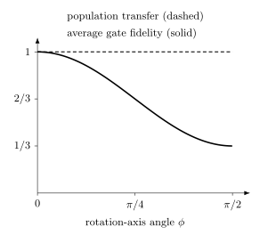
One input state does not characterize a gate. Both curves describe the same family of ideal $\pi$ pulses; only the gate-sensitive objective detects the wrong rotation axis.

The same issue appears with experimental rewards. Readout errors, leakage, spectator qubits and drift may affect the score. Choose measurements sensitive to the intended operation, and describe which physical effects they can miss. Metrics for Quantum Hardware explains what common characterization protocols estimate.

Choose what the optimizer can change

A control vector $\boldsymbol\alpha$ might contain sampled amplitudes, spline knots, pulse widths or a few corrections to an analytic pulse. For $m$ channels and $N$ independent samples per channel, there are $mN$ real variables if each channel is real valued. Independent in-phase and quadrature amplitudes count as separate real channels.

Many variables make the pulse family flexible, but also make noisy experimental search expensive. A compact family can be easier to tune and interpret. Its limitation is expressiveness: no optimizer can find a pulse excluded by the chosen family. Increasing the dimension of a nested family cannot worsen the exact best attainable training loss, but the result of a finite search or its performance on new data can worsen.

For uncertain device parameters $\theta$, a typical objective is

$$J(\boldsymbol\alpha) =\mathbb E_\theta[L(\boldsymbol\alpha,\theta)] +\lambda C(\boldsymbol\alpha).$$

Here $L$ measures the physical error and $C$ penalizes a chosen resource, such as integrated power. The weight $\lambda$ must have the units needed to combine the terms. A penalty expresses a tradeoff; it does not enforce a strict bound.

For example, an amplitude limit requires

$$|u(t;\boldsymbol\alpha)|\leq A_{\max}.$$

Clipping an infeasible pulse after optimization changes its dynamics. Either search only feasible controls or include the actual clipping transformation in every simulated objective evaluation. Smooth approximations can help compute gradients, but the final pulse must be checked with the actual transformation. Filtering, quantization and sampling can likewise change the result. See the worked pulse-response example in Pulse-Level Control.

Match the search method to the available information

Method	Useful information	Main limitation
GRAPE or other adjoint gradients	differentiable dynamics and objective	model and numerical errors affect the gradient
Krotov methods	dynamics and a suitable variational functional	monotonicity depends on the formulation and discretization
Compact-basis search, including CRAB	repeated objective evaluations	a restricted basis can exclude good pulses
Bayesian or direct search	noisy experimental scores in a modest dimension	limited evaluations and drift
Policy optimization, including reinforcement learning	trajectories, observations and rewards	reward quality, sample cost and controller timing

These are useful starting points, not disjoint categories. Compact parameters can be optimized with gradients, and a hardware score can support estimated gradients such as simultaneous perturbations. The choice concerns the cost and reliability of information, not simply whether a derivative exists on paper.

Gradients from a dynamical model

GRAPE divides a pulse into time slices and uses forward and backward propagation to compute how the objective changes with the controls. This avoids one complete propagation for every parameter perturbation, although local matrix derivatives and memory still have a cost. Khaneja and colleagues developed this approach for coupled-spin control.

Check a gradient by perturbing a small selection of parameters or a random direction. For a smooth numerical objective,

$$\frac{J(\boldsymbol\alpha+h\boldsymbol v) -J(\boldsymbol\alpha-h\boldsymbol v)}{2h} \approx\boldsymbol v\cdot\nabla J.$$

Try several $h$ values. Large steps have truncation error; excessively small steps amplify roundoff or solver error. A successful check establishes a derivative of the numerical model. It does not establish that the model describes the device. Also refine the propagation time step, expand any truncated Hilbert space and test a more accurate delivery model where relevant.

Krotov methods use a variational construction to update the field. Suitable formulations guarantee monotonic improvement of their functional under stated assumptions. Coarse time grids, ad hoc clipping and altered penalties can invalidate that conclusion. Monotonic improvement also does not prove a global optimum. Goerz and colleagues explain the method and its discretization in their implementation paper.

Search in a reduced pulse basis

CRAB uses a finite set of basis functions, often with randomly chosen frequencies. One possible additive correction is

$$\begin{aligned} u(t)&=u_0(t)+s(t)\sum_{k=1}^{K}c_k(t),\\ c_k(t)&=a_k\sin(\omega_k t)+b_k\cos(\omega_k t). \end{aligned}$$

The envelope $s(t)$ can make the correction vanish at the endpoints. A search over the $2K$ coefficients replaces a search over every sample. CRAB was introduced by Caneva and colleagues; dCRAB refreshes the basis directions between searches, as developed by Rach and colleagues.

Bounding the listed frequencies alone does not make the delivered finite pulse strictly band limited. Multiplication by $s(t)$ convolves spectra, and time truncation, sampling and clipping add further spectral structure. Check the actual filtered waveform against the physical spectral requirement. A smooth pulse with little power outside an allowed band is a meaningful target; an exactly time-limited nonzero pulse cannot also have compact frequency support.

Search using experimental scores

Bayesian optimization models an unknown score and chooses new points by balancing predicted performance against uncertainty. Direct and evolutionary methods use other rules for proposing and comparing candidates. They can be useful when a simulator is inaccurate, especially in a low-dimensional pulse family. Their performance depends on noise, parameter scaling, drift and the evaluation budget; no family is uniformly best.

A practical combination is to optimize a pulse in simulation, then tune a few amplitude, phase or detuning corrections on the device. Egger and Wilhelm’s adaptive hybrid approach illustrates this idea. Kelly and colleagues used randomized benchmarking as a control-optimization signal. Such a score keeps the assumptions of its characterization protocol; optimization does not make it a complete description of the gate.

Fixed pulses and feedback policies

Tuning a fixed waveform through repeated experiments differs from choosing an action during a single experiment. In the latter case a policy can depend on the observation history:

$$a_t\sim\pi_{\boldsymbol\phi}(\,\cdot\mid o_{\leq t}).$$

The observations may be discrete outcomes or continuous measurement signals. Only observations already available to the controller may influence its next action; latency determines which information is usable.

Reinforcement learning can optimize such a policy by maximizing a return,

$$J_{\mathrm{RL}}(\boldsymbol\phi) =\mathbb E\left[\sum_{t=0}^{T}\gamma^t r_t\right],$$

where the sum is over decision steps and $\gamma$ discounts later rewards. It can also learn a fixed open-loop sequence, so using reinforcement learning does not by itself imply measurement feedback. Sivak and colleagues provide an experimental example of learning control from measurement-based rewards. For a fixed waveform and terminal score, compare against simpler pulse search methods under the same measurement budget. For live feedback, test noisy records and delayed observations as well as the average return. See Measurement-Based Feedback for the stochastic dynamics.

Robustness means performance under specified changes

A pulse can be insensitive to static detuning but sensitive to rapid frequency noise. State whether each uncertain parameter is fixed during a pulse, varies between shots or changes during the evolution. Include relevant correlations: independently sampling parameters does not test a correlated drift model.

The mean loss $\mathbb E[L]$ describes typical weighted performance; the worst-case loss $\sup_{\theta\in\Theta}L$ describes an entire uncertainty set. Tail-risk objectives emphasize large losses. Their definitions, including discrete tail probabilities, are explained in Error-Aware Compilation. A maximum over finitely many sampled parameters is only a lower bound on the worst-case loss over a continuous set unless further bounds are established.

Test a fixed optimized pulse on new uncertainty points and independent device measurements. More points on a deterministic grid can reveal behavior between training points, but do not by themselves prove performance everywhere. For statistical generalization, the test distribution must represent the claimed operating conditions. Extrapolation beyond those conditions is a separate test.

Count measurements and compare fairly

An experimental score may average several circuits and many repetitions. If $N_c$ candidates each use $N_s$ settings and $n$ shots per setting, their basic measurement cost is

$$B=N_cN_sn.$$

Add measurements of reference pulses, repeated evaluations and final testing. Wall-clock time also includes resets, uploads, queueing and analysis. Comparing optimizer iterations is insufficient when each method uses a different number of physical measurements.

For a Bernoulli success probability estimated from $n$ independent shots,

$$\operatorname{SE}(\widehat p) =\sqrt{\frac{p(1-p)}{n}}.$$

Near $p=1/2$, a difference of $0.01$ between two independent equally sized batches has standard error at most $\sqrt{1/(2n)}$. Achieving a standard error of $0.005$ therefore requires $n=20{,}000$ shots per candidate in this worst-variance case. This is a precision calculation, not a full hypothesis test or power guarantee. Drift and correlated shots require a different model.

Repeatedly measuring the current reference pulse helps distinguish improvement from drift. Randomize or interleave comparisons and retain the time dependence. Fresh test data can use the same metric as training; complementary metrics are useful when the training score omits phases, leakage or other relevant effects. Selecting the best of many noisy candidates makes its training score optimistic, so evaluate the chosen pulse again without tuning to those data.

Keep enough information to reproduce the physical comparison: the pulse sent to the device, model and control conventions, parameter bounds, objective, search settings, measurement counts and independent test results. The result supports performance in the tested context; it does not establish optimality among all possible controls or robustness on every device.

Exercises

1. Distinguish two loops

An optimizer runs a fixed pulse, measures its final state and changes the pulse for the next batch. Does the pulse implement measurement feedback?

Solution

No. The search uses feedback between experiments, but each pulse is fixed within its experiment. Measurement feedback would choose a later action in the same run using an earlier measurement outcome.

2. Count the query budget

A search evaluates 36 candidates, each with 8 circuit settings and 2,000 shots per setting. Reference measurements add 10% of this candidate shot count. Ignoring integer rounding, find the total.

Solution

The candidates use $36\times8\times2{,}000=576{,}000$ shots. Adding 10% gives 633,600. This assumes the overhead is 10% of candidate shots; if instead reference shots were 10% of the final total, the total would be $576{,}000/0.9=640{,}000$.

3. Choose a useful first search

A differentiable simulator has 1,200 waveform variables. Only fifty final candidate evaluations are available on the device. How can these resources be combined?

Solution

Use adjoint gradients for the large simulated search, with the physical bounds and uncertainty model included. Reserve device evaluations for independent comparison and a small correction family if needed. Fifty noisy evaluations are generally insufficient to explore 1,200 unrelated control variables without strong additional structure.

4. An amplitude bound limits the task

Let $H(t)=u(t)X/2$, with $\hbar=1$, real $u$ and $|u|\leq A_{\max}$. Starting in $|0\rangle$, show that perfect transfer to $|1\rangle$ needs $T\geq\pi/A_{\max}$. Find the best transfer probability when $A_{\max}T=\pi/2$.

Solution

All Hamiltonians commute, so the rotation angle is $\vartheta=\int_0^T u(t)\,dt$, with $|\vartheta|\leq A_{\max}T$. The transfer probability is $\sin^2(\vartheta/2)$. Its first unit maximum occurs at $|\vartheta|=\pi$, giving the bound. For the stated shorter duration, the best probability is $\sin^2(\pi/4)=1/2$, attained by a constant maximal amplitude. More optimizer iterations cannot remove this physical restriction. This bound is specific to the stated single-axis Hamiltonian.

5. Test between training points

A pulse is optimized at detunings $\{-2,-1,0,1,2\}\,\mathrm{MHz}$. Does a maximum loss of $10^{-3}$ at these points bound its loss throughout the interval? Suggest a further test.

Solution

No; a larger loss may occur between them. Evaluate the fixed pulse on finer or shifted points, such as half-integer detunings inside the interval, and on joint amplitude/detuning perturbations relevant to the device. Even a finer finite grid is not a rigorous interval bound without additional information, such as a justified bound on how rapidly the loss can vary. Points outside $[-2,2]\,\mathrm{MHz}$ test extrapolation separately.

6. Detect the wrong rotation axis

For $U_\phi$ above, compute the fidelity for the input $|+\rangle$ relative to the intended $X$ gate. Evaluate it and the average gate fidelity at $\phi=\pi/4$.

Solution

The target leaves $|+\rangle$ unchanged up to a global phase. Since $\langle+|Y|+\rangle=0$ and $\langle+|X|+\rangle=1$, the input fidelity is $|\langle+|U_\phi|+\rangle|^2=\cos^2\phi$. It is $1/2$ at $\pi/4$, while $F_{\mathrm{avg}}=2/3$. Both detect an error that the $|0\rangle$ population-transfer experiment misses.

7. Check a derivative

For a resonant pulse of angle $\vartheta$, the transfer loss is $L(\vartheta)=\cos^2(\vartheta/2)$. Find its derivative and compare it with a central difference at $\vartheta=\pi/2$.

Solution

The derivative is $L'=-\sin\vartheta/2$, giving $-1/2$ at $\pi/2$. The central difference is $-\sin h/(2h)$, which approaches $-1/2$ with error $h^2/12+O(h^4)$. A finite-difference test can expose a missing sign or scale factor, provided the propagation and arithmetic errors are smaller than the perturbation signal.

8. A penalty is not a hard constraint

Minimize $J(a)=(a-2)^2+\lambda\max(0,a-1)^2$ for finite $\lambda>0$. Does its minimizer satisfy the intended bound $a\leq1$?

Solution

For $a>1$, stationarity gives

$$a_* =\frac{2+\lambda}{1+\lambda} =1+\frac{1}{1+\lambda}.$$

This is the unique minimum of the convex objective and exceeds one for every finite $\lambda$. Direct constrained minimization instead gives $a=1$. Increasing the penalty reduces the violation but does not prove feasibility.

9. How many shots resolve a change?

Two independent Bernoulli batches each have $n=5{,}000$ shots. Near success probability one half, estimate the standard error of their difference. How much must $n$ grow to halve that error?

Solution

The variances add, so the standard error is $\sqrt{(1/4+1/4)/5{,}000}=0.01$. It falls as $n^{-1/2}$; four times as many shots, 20,000 per batch, halve it. A 0.01 observed difference with the smaller batches is only one standard error, not a convincing improvement by itself. Adaptive candidate selection adds a further reason for a fresh test.

10. What a frequency cutoff leaves out

Take $s(t)=\sin^2(\pi t/T)$ and multiply it by $\cos(\omega t)$ on $0\leq t\leq T$. Which frequencies appear before this finite-time window is applied? Is the full pulse strictly band limited?

Solution

Writing $\nu=2\pi/T$ gives

$$s(t)\cos(\omega t) ={}\tfrac12\cos(\omega t) -\tfrac14\cos[(\omega+\nu)t] -\tfrac14\cos[(\omega-\nu)t].$$

Even before finite-time truncation, the envelope introduces shifted frequencies. Restricting the function to a finite interval broadens its spectrum further. Endpoint smoothness reduces high-frequency tails but does not make their support compact.

References

• T. Caneva, T. Calarco, and S. Montangero, “Chopped random-basis quantum optimization,” Physical Review A 84, 022326 (2011), doi:10.1103/PhysRevA.84.022326.
• D. J. Egger and F. K. Wilhelm, “Adaptive hybrid optimal quantum control for imprecisely characterized systems,” Physical Review Letters 112, 240503 (2014), doi:10.1103/PhysRevLett.112.240503.
• M. H. Goerz et al., “Krotov: a Python implementation of Krotov’s method for quantum optimal control,” SciPost Physics 7, 080 (2019), doi:10.21468/SciPostPhys.7.6.080.
• J. Kelly et al., “Optimal quantum control using randomized benchmarking,” Physical Review Letters 112, 240504 (2014), doi:10.1103/PhysRevLett.112.240504.
• N. Khaneja, T. Reiss, C. Kehlet, T. Schulte-Herbrüggen, and S. J. Glaser, “Optimal control of coupled spin dynamics: design of NMR pulse sequences by gradient ascent algorithms,” Journal of Magnetic Resonance 172, 296–305 (2005), doi:10.1016/j.jmr.2004.11.004.
• M. A. Nielsen, “A simple formula for the average gate fidelity of a quantum dynamical operation,” Physics Letters A 303, 249–252 (2002), arXiv:quant-ph/0205035.
• N. Rach, M. M. Müller, T. Calarco, and S. Montangero, “Dressing the chopped-random-basis optimization: a bandwidth-limited access to the trap-free landscape,” Physical Review A 92, 062343 (2015), doi:10.1103/PhysRevA.92.062343.
• V. V. Sivak, A. Eickbusch, H. Liu, B. Royer, I. Tsioutsios, and M. H. Devoret, “Model-free quantum control with reinforcement learning,” Physical Review X 12, 011059 (2022), doi:10.1103/PhysRevX.12.011059.