Partial Trace

The partial trace removes one tensor factor from an operator while retaining exactly the information needed for the other factor. For a bipartite density operator $\rho_{AB}$,

$$\rho_A = \operatorname{Tr}_B\rho_{AB}.$$

Required background. Density Operators supplies the state and trace language, and Entangled States supplies the subsystem interpretation. Familiarity with finite-dimensional product bases and operator matrices is assumed.

Partial trace as an operator map

Work first in finite dimensions, where every operator has a trace. For infinite-dimensional spaces, take $X_{AB}$ trace class and test against bounded local operators; the basis sums then converge in trace norm. In particular, the identity on an infinite-dimensional factor cannot simply be traced to a finite scalar.

The defining requirement is that discarding $B$ must preserve every prediction for a measurement confined to $A$:

$$\operatorname{Tr}_A\!\left[(\operatorname{Tr}_B X_{AB})M_A\right] =\operatorname{Tr}_{AB}\!\left[X_{AB}(M_A\otimes I_B)\right].$$

For $X_{AB}=\rho_{AB}$, both sides are the expectation of the same local observable $M_A$. The identity also holds for general bounded $M_A$, by linearity. It fixes which factor remains before any matrix indices are contracted. The reduced-state interpretation explains what local predictions leave out; here we derive the contraction rules used to calculate them.

To recover the matrix elements, choose $M_A=|k\rangle\langle i|$ in orthonormal product bases. Expanding the full trace gives

$$\begin{aligned} (\operatorname{Tr}_B X_{AB})_{ik} &=\operatorname{Tr}_{AB}\!\left[X_{AB}(|k\rangle\langle i|\otimes I_B)\right]\\ &=\sum_{a,b}\langle a,b|X_{AB}|k,b\rangle\langle i|a\rangle\\ &=\sum_b\langle i,b|X_{AB}|k,b\rangle. \end{aligned}$$

Thus the local-prediction requirement determines every matrix element uniquely. Although $|k\rangle\langle i|$ need not be Hermitian, it is a complex linear combination of Hermitian observables, so using it introduces no extra physical assumption.

Let

$$X_{AB} \in \mathcal L \bigl( \mathcal H_A\otimes\mathcal H_B \bigr).$$

The full trace returns a scalar:

$$\operatorname{Tr}_{AB}X_{AB} \in \mathbb C.$$

The partial trace returns an operator on the subsystem that remains:

$$\operatorname{Tr}_B X_{AB} \in \mathcal L(\mathcal H_A).$$

If $d_A$ and $d_B$ are finite, the map changes a $(d_A d_B)\times(d_A d_B)$ matrix into a $d_A\times d_A$ matrix. Tracing out $A$ instead gives a $d_B\times d_B$ matrix.

The partial trace is linear, positive, and trace-preserving:

$$\operatorname{Tr}_A \left( \operatorname{Tr}_B X_{AB} \right) = \operatorname{Tr}_{AB}X_{AB}.$$

When $X_{AB}=\rho_{AB}$ is a density operator, the result is therefore a normalized positive operator: the reduced state of subsystem $A$.

Tracing out $B$ is not the same as projecting $B$ onto one selected state. It is a sum over a complete orthonormal basis of the subsystem being ignored.

Basis Calculation

Choose an orthonormal basis $\{\lvert b\rangle_B\}$. The partial trace over $B$ can be written as a sum of contractions. Define

$$R_b \equiv I_A\otimes{}_B\langle b\rvert, \qquad R_b^\dagger = I_A\otimes\lvert b\rangle_B.$$

Then

$$\operatorname{Tr}_B X_{AB} = \sum_b R_b X_{AB}R_b^\dagger.$$

Each term inserts a bra and ket on subsystem $B$, leaving an operator on subsystem $A$.

Why the result is basis-independent

Let another orthonormal basis be related by a unitary matrix:

$$\lvert\beta\rangle = \sum_b U_{b\beta}\lvert b\rangle.$$

Define $R_\beta=I_A\otimes\langle\beta\rvert$ in the new basis.

Using

$$\sum_\beta U_{b\beta}^*U_{c\beta} = \delta_{bc},$$

the basis sum becomes

$$\begin{aligned} \sum_\beta R_\beta X_{AB}R_\beta^\dagger &= \sum_{b,c} \delta_{bc}\, R_b X_{AB}R_c^\dagger\\ &= \sum_b R_b X_{AB}R_b^\dagger. \end{aligned}$$

The basis formula is a calculation device; the resulting operator does not depend on which orthonormal basis was used.

Tensor-Product and Dyad Rules

For a simple tensor of operators,

$$\operatorname{Tr}_B \bigl( X_A\otimes Y_B \bigr) = X_A\,\operatorname{Tr}Y_B.$$

Linearity then handles every finite sum of tensor products. The most useful elementary case is the dyad rule:

$$\operatorname{Tr}_B \left( \lvert i\rangle\langle k\rvert_A \otimes \lvert j\rangle\langle\ell\rvert_B \right) = \delta_{j\ell}\, \lvert i\rangle\langle k\rvert_A.$$

This is just the ordinary trace on the $B$ factor:

$$\operatorname{Tr} \left( \lvert j\rangle\langle\ell\rvert \right) = \langle\ell\vert j\rangle = \delta_{j\ell}.$$

The cross terms in the subsystem being traced out vanish when their basis labels are different.

Coefficient and Block Rules

In product bases, write

$$\rho_{AB} = \sum_{i,k,j,\ell} \rho_{ij,k\ell} \, \lvert i\rangle\langle k\rvert_A \otimes \lvert j\rangle\langle\ell\rvert_B.$$

Then

$$\rho_A = \operatorname{Tr}_B\rho_{AB} = \sum_{i,k} \left( \sum_j \rho_{ij,kj} \right) \lvert i\rangle\langle k\rvert_A.$$

Equivalently, the matrix elements of the reduced state are

$$(\rho_A)_{ik} = \sum_j \rho_{ij,kj}.$$

The repeated $B$ label $j$ is the one being summed. The $A$ labels $i,k$ remain because the result is still an operator on $\mathcal H_A$.

Block-matrix view

With the $A$ index first and the $B$ index changing fastest, regard $X_{AB}$ as a $d_A\times d_A$ array of $d_B\times d_B$ blocks:

$$X_{AB} = \begin{pmatrix} X_{00}^{(B)}&\cdots&X_{0,d_A-1}^{(B)}\\ \vdots&\ddots&\vdots\\ X_{d_A-1,0}^{(B)}&\cdots&X_{d_A-1,d_A-1}^{(B)} \end{pmatrix}.$$

Tracing out $B$ takes the ordinary trace of every block:

$$\operatorname{Tr}_B X_{AB} = \sum_{i,k} \operatorname{Tr} \left( X_{ik}^{(B)} \right) \lvert i\rangle\langle k\rvert_A.$$

By contrast, tracing out $A$ sums the diagonal $B$-space blocks:

$$\operatorname{Tr}_A X_{AB} = \sum_i X_{ii}^{(B)}.$$

These recipes assume the declared $A$-first ordering. If a matrix uses a different flattened product basis, reorder it before applying a memorized block rule.

Pure-State Shortcut

Suppose

$$\lvert\Psi\rangle = \sum_{i,j}C_{ij}\, \lvert i\rangle_A\otimes\lvert j\rangle_B,$$

where $C$ is the $d_A\times d_B$ coefficient matrix with $A$ indexing rows. Then

$$\rho_A=CC^\dagger, \qquad \rho_B=C^{\mathsf T}C^*.$$

For example,

$$\begin{aligned} (\rho_A)_{ik} &= \sum_j C_{ij}C_{kj}^*\\ &= \sum_j \rho_{ij,kj}. \end{aligned}$$

This is exactly the coefficient rule above. It avoids constructing the full $(d_A d_B)\times(d_A d_B)$ matrix $\lvert\Psi\rangle\langle\Psi\rvert$.

Moving operators through a partial trace

Operators on the retained factor pull outside on the same side:

$$\operatorname{Tr}_B[(M_A\otimes I)X]=M_A\operatorname{Tr}_B X, \qquad \operatorname{Tr}_B[X(M_A\otimes I)]=(\operatorname{Tr}_B X)M_A.$$

Operators on the discarded factor can be moved cyclically:

$$\operatorname{Tr}_B[(I\otimes N_B)X] =\operatorname{Tr}_B[X(I\otimes N_B)].$$

These are finite-dimensional identities, or trace-class/bounded identities in infinite dimensions. The latter follows by expanding the summed $B$ indices. It is essential in proving that remote trace-preserving operations leave local statistics unchanged.

A partial trace is not fully cyclic. For $X=|00\rangle\langle00|$ and $M_A=\sigma_x$, placing $M_A\otimes I$ on the left gives $|1\rangle\langle0|$, while placing it on the right gives $|0\rangle\langle1|$. The untraced $A$ factors retain their order.

Two-Qubit Matrix Rule

For two qubits in the ordered product basis

$$\lvert00\rangle,\; \lvert01\rangle,\; \lvert10\rangle,\; \lvert11\rangle,$$

the reduced density matrix of qubit $A$ has entries

$$\rho_A = \begin{pmatrix} \rho_{00,00}+\rho_{01,01} & \rho_{00,10}+\rho_{01,11} \\ \rho_{10,00}+\rho_{11,01} & \rho_{10,10}+\rho_{11,11} \end{pmatrix}.$$

The convention is

$$\rho_{ij,k\ell} = \langle i,j\rvert \rho_{AB} \lvert k,\ell\rangle.$$

The pair $(i,j)$ labels the matrix row and $(k,\ell)$ labels the matrix column. For example,

$$\rho_{01,11} = \langle0,1\rvert \rho_{AB} \lvert1,1\rangle.$$

This rule says: keep the $A$ labels and sum over matching $B$ labels.

Bell State Example

For

$$\lvert\Phi^+\rangle = \frac{ \lvert00\rangle+\lvert11\rangle }{\sqrt2},$$

the density matrix in the same ordered basis is

$$\rho_{AB} = \frac{1}{2} \begin{pmatrix} 1 & 0 & 0 & 1 \\ 0 & 0 & 0 & 0 \\ 0 & 0 & 0 & 0 \\ 1 & 0 & 0 & 1 \end{pmatrix}.$$

Using the two-qubit rule,

$$\begin{aligned} (\rho_A)_{00} &= \rho_{00,00}+\rho_{01,01} = \frac{1}{2}, \\ (\rho_A)_{11} &= \rho_{10,10}+\rho_{11,11} = \frac{1}{2}, \\ (\rho_A)_{01} &= \rho_{00,10}+\rho_{01,11} = 0, \\ (\rho_A)_{10} &= \rho_{10,00}+\rho_{11,01} = 0. \end{aligned}$$

Therefore

$$\rho_A = \frac{1}{2} \begin{pmatrix} 1 & 0 \\ 0 & 1 \end{pmatrix} = \frac{I_A}{2}.$$

The same calculation gives $\rho_B=I_B/2$.

Same marginal from a different joint state

The separable, classically correlated state

$$\rho_{\mathrm{cc}} = \frac12 \lvert00\rangle\langle00\rvert + \frac12 \lvert11\rangle\langle11\rvert$$

has matrix

$$\rho_{\mathrm{cc}} = \frac12 \begin{pmatrix} 1&0&0&0\\ 0&0&0&0\\ 0&0&0&0\\ 0&0&0&1 \end{pmatrix}.$$

The same block trace gives

$$\operatorname{Tr}_B\rho_{\mathrm{cc}} = \frac12 I_A.$$

The Bell state and $\rho_{\mathrm{cc}}$ have the same reduced state but different joint coherence and correlations. This illustrates directly that the partial trace is many-to-one.

Checking a calculation

For a density operator, the output must have the retained dimension, be Hermitian and positive, and have trace one. These checks catch many indexing mistakes, but not every wrong subsystem choice: tracing the wrong qubit can still give a valid density matrix.

Compare a local expectation from both descriptions, using an observable that distinguishes the factors. For $|01\rangle$, the correct retained $A$ state has $\langle Z_A\rangle=+1$, whereas the $B$ state has $\langle Z_B\rangle=-1$. A Bell pair alone is a weak test because its two marginals coincide.

Closing only the discarded indices

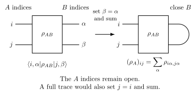
A partial trace closes only the discarded subsystem’s pair of indices. The remaining indices label matrix elements of $\rho_A$; closing them as well would produce the scalar $\operatorname{Tr}\rho_{AB}=1$.

In tensor-network notation, an operator on $AB$ has an input and output leg for $A$ and an input and output leg for $B$. Taking $\operatorname{Tr}_B$ connects the $B$ output leg back to the $B$ input leg and sums over that internal label. The $A$ input and output legs remain open, so the result is an operator on $A$.

This picture is often the cleanest way to remember the operation: a trace closes a pair of matching legs. A partial trace closes only the legs belonging to the subsystem being discarded.

Multiple Subsystems

For three subsystems,

$$\mathcal H_{ABC} = \mathcal H_A\otimes\mathcal H_B\otimes\mathcal H_C,$$

one may trace over more than one subsystem:

$$\rho_A = \operatorname{Tr}_{BC}\rho_{ABC} = \operatorname{Tr}_B \bigl( \operatorname{Tr}_C\rho_{ABC} \bigr).$$

Partial traces over distinct factors commute:

$$\operatorname{Tr}_B\operatorname{Tr}_C\rho_{ABC} = \operatorname{Tr}_C\operatorname{Tr}_B\rho_{ABC}.$$

The order of tensor factors still matters for index contractions. If the register order is $A,B,C$, then tracing out the middle subsystem means summing over the middle input-output pair, not simply deleting adjacent rows and columns of a matrix.

Computational Implementation

For finite-dimensional systems, the safest implementation is to reshape the matrix into a tensor with one row index and one column index for each subsystem.

For a bipartite operator with dimensions $d_A$ and $d_B$, use components

$$X_{a b, a' b'}.$$

Then

$$(\operatorname{Tr}_B X)_{a a'} = \sum_{b=0}^{d_B-1} X_{a b, a' b}.$$

In array language, this is a contraction over the $B$ row index and the $B$ column index. A good implementation should make the subsystem dimensions and basis ordering explicit rather than inferring them from the total matrix size.

For an $A$-first, $B$-fast row-major array, reshape to $(d_A,d_B,d_A,d_B)$ and contract axes 1 and 3 (zero-based). A column-major language needs a matching reshape/permutation convention. Computational notebooks gives executable examples. Check the result using a stated floating-point tolerance; do not silently renormalize a substantial trace error.

Common pitfalls

A partial trace is not a projection. One bra–ket contraction selects a branch; summing a complete basis gives the marginal.

The same array can represent different factor orders. Declare the dimensions and flattened order before using blocks or reshaping.

Trace preservation is not division by the discarded dimension. In particular, $\operatorname{Tr}_B I_{AB}=d_B I_A$. Density operators remain normalized because the input already has unit trace.

References

• Heinz-Peter Breuer and Francesco Petruccione, The Theory of Open Quantum Systems, Oxford University Press, 2002, chapter 2.
• Michael A. Nielsen and Isaac L. Chuang, Quantum Computation and Quantum Information, 10th anniversary ed., Cambridge University Press, 2010, sections 2.4–2.5.
• John Watrous, The Theory of Quantum Information, Cambridge University Press, 2018, section 2.1.3, especially equations (2.32)–(2.34), for product and component forms of reduction. Author-hosted chapter.

Exercises

1. Compute

$$\operatorname{Tr}_B \left( |0\rangle\langle1|_A \otimes |1\rangle\langle1|_B \right).$$

Solution

The trace of $|1\rangle\langle1|_B$ is $1$, so

$$\operatorname{Tr}_B \left( |0\rangle\langle1|_A \otimes |1\rangle\langle1|_B \right) = |0\rangle\langle1|_A.$$

2. Compute

$$\operatorname{Tr}_B \left( |0\rangle\langle1|_A \otimes |0\rangle\langle1|_B \right).$$

Solution

The trace of $|0\rangle\langle1|_B$ is $\langle1|0\rangle=0$, so the result is

$$0.$$

3. Trace out qubit $B$ from the product state $|01\rangle\langle01|$.

Solution

Write

$$|01\rangle\langle01| = |0\rangle\langle0|_A \otimes |1\rangle\langle1|_B.$$

Taking the trace over $B$ gives

$$\operatorname{Tr}_B(|01\rangle\langle01|) = |0\rangle\langle0|_A.$$

4. In register order $A,B,C$, trace out the middle qubit from $|\psi\rangle=(|000\rangle+|101\rangle)/\sqrt2$. Why do the cross terms survive?

Solution

Both terms have $B=0$, so every $B$ overlap equals $\langle0|0\rangle=1$. The retained state is

$$\rho_{AC}=|\Phi^+\rangle_{AC}\langle\Phi^+|.$$

The off-diagonal term $|000\rangle\langle101|$ becomes $|00\rangle_{AC}\langle11|$. Unequal retained labels do not kill a term; only the labels on the traced factor are contracted.

5. If $\rho_A=\operatorname{Tr}_B\rho_{AB}$, what operator on $AB$ corresponds to measuring an observable $M_A$ only on subsystem $A$?

Solution

The corresponding composite-system observable is

$$M_A\otimes I_B.$$

The defining expectation-value property is

$$\operatorname{Tr}_{AB} \left[ \rho_{AB}(M_A\otimes I_B) \right] = \operatorname{Tr}_A(\rho_A M_A).$$

6. Verify trace compatibility for a product operator:

$$\operatorname{Tr}_A \left[ \operatorname{Tr}_B \bigl( X_A\otimes Y_B \bigr) \right] = \operatorname{Tr}_{AB} \bigl( X_A\otimes Y_B \bigr).$$

Why does the result extend to finite sums of product operators?

Solution

First trace over $B$:

$$\operatorname{Tr}_B \bigl( X_A\otimes Y_B \bigr) = X_A\,\operatorname{Tr}Y_B.$$

Then

$$\begin{aligned} \operatorname{Tr}_A \left[ X_A\,\operatorname{Tr}Y_B \right] &= \operatorname{Tr}X_A\, \operatorname{Tr}Y_B\\ &= \operatorname{Tr}_{AB} \bigl( X_A\otimes Y_B \bigr). \end{aligned}$$

Both the full trace and partial trace are linear, so the identity extends term by term to finite sums.

7. Use the coefficient-matrix shortcut for

$$\lvert\Psi\rangle = \frac{ 2\lvert00\rangle +\lvert01\rangle +\lvert11\rangle }{\sqrt6}.$$

Compute both reduced states and check their traces.

Solution

The coefficient matrix is

$$C = \frac{1}{\sqrt6} \begin{pmatrix} 2&1\\ 0&1 \end{pmatrix}.$$

Therefore

$$\rho_A = CC^\dagger = \frac16 \begin{pmatrix} 5&1\\ 1&1 \end{pmatrix},$$

and

$$\rho_B = C^{\mathsf T}C^* = \frac16 \begin{pmatrix} 4&2\\ 2&2 \end{pmatrix}.$$

Both have unit trace:

$$\operatorname{Tr}\rho_A = \operatorname{Tr}\rho_B =1.$$

8. For the Bell state $\lvert\Phi^+\rangle$, compare (a) tracing out $B$, (b) projecting onto the outcome $B=0$, and (c) performing a complete computational-basis measurement on $B$ and discarding its outcome. Identify the output object in each case and explain why (a) and (c) give the same local state on $A$ even though they are different operations on the joint system.

The expressions for (a) and the unnormalized branch in (b) are

$$\operatorname{Tr}_B \left( \lvert\Phi^+\rangle\langle\Phi^+\rvert \right)$$

and

$$\bigl( I_A\otimes{}_B\langle0\rvert \bigr) \lvert\Phi^+\rangle\langle\Phi^+\rvert \bigl( I_A\otimes\lvert0\rangle_B \bigr).$$

Solution

The partial trace sums over a complete basis of $B$ and gives

$$\operatorname{Tr}_B \left( \lvert\Phi^+\rangle\langle\Phi^+\rvert \right) = \frac12 I_A.$$

The second expression selects only the $B=0$ component:

$$\bigl( I_A\otimes{}_B\langle0\rvert \bigr) \lvert\Phi^+\rangle\langle\Phi^+\rvert \bigl( I_A\otimes\lvert0\rangle_B \bigr) = \frac12 \lvert0\rangle\langle0\rvert_A.$$

It is an unnormalized conditional operator with trace $1/2$, the probability of the selected outcome. After normalization it becomes $\lvert0\rangle\langle0\rvert_A$.

For (c), the nonselective measurement produces the joint state

$$\rho'_{AB} = \frac12\lvert00\rangle\langle00\rvert + \frac12\lvert11\rangle\langle11\rvert.$$

This operation removes joint coherence and therefore differs from merely computing a reduced state. Nevertheless, $\operatorname{Tr}_B\rho'_{AB}=I_A/2$, the same local state obtained in (a). Projection selects one branch, nonselective measurement changes the joint state and averages all branches, and partial trace extracts the local state without specifying a measurement.