Circuit Model

The quantum circuit model represents a computation as an ordered network of quantum systems and operations. Quantum wires carry subsystem state from one operation to the next. Gates act on one or more wires. Measurements produce classical records, and those records may control later operations. A complete circuit specification also states how inputs are prepared, what counts as output, and which resources are being counted.

In the ideal unitary form, an $n$-qubit input is transformed by a sequence of local unitary gates and measured at the end. The more general and operationally complete form allows mixed states, channels, mid-circuit measurements, discarding, reset, and classical feedforward. It is then a composition of quantum channels or instruments rather than one unitary matrix.

To calculate what a diagram does, fix the wire order, operation sequence, input state and output being read. Counting its cost additionally requires a gate set, connectivity and scheduling rules.

Helpful background. Qubits and encodings explains registers; density operators treats mixed states and conditional outputs; tensor-product ordering translates between matrix and wire conventions.

Registers and Basis Conventions

An $n$-qubit register $Q=Q_1\cdots Q_n$ has Hilbert space

$$\mathcal H_Q = \bigotimes_{j=1}^{n} \mathbb C^2.$$

Choose and state the tensor-factor order. This page uses

$$\lvert x_1x_2\cdots x_n\rangle \equiv \lvert x_1\rangle_{Q_1} \otimes \lvert x_2\rangle_{Q_2} \otimes\cdots\otimes \lvert x_n\rangle_{Q_n},$$

where $x_j\in\{0,1\}$. The computational basis has $2^n$ vectors, but this exponential dimension does not imply that a circuit can read out $2^n$ independent classical values.

Software libraries disagree about bitstring display order, integer endianness, and which matrix factor corresponds to the top wire. Those are coordinate conventions, not physical differences. A trustworthy calculation declares:

1. the top-to-bottom wire order;
2. the tensor-product order;
3. how a displayed bitstring maps to an integer;
4. whether outcome strings are printed in diagram order or reversed.

For example, in the tensor order above, $|100\rangle$ has its first qubit excited, regardless of whether software prints the associated classical bits as 100 or 001. Follow the explicit mapping rather than inferring it from an integer label.

Registers need not be qubits. A qudit wire may carry $\mathbb C^d$, a bosonic wire may carry a mode, and an encoded logical wire may denote a code subspace spread over many physical systems. The circuit grammar survives, but the allowed gates, measurements, leakage modes, and resource units change.

The chapter guide links the mode, bosonic-encoding and topological computation models. Each specifies how its physical systems represent logical registers.

What a Wire Means

A quantum wire denotes the identity connection between two operation ports. It says that the output subsystem of one operation is the input subsystem of the next. It does not assert that the wire carries a hidden classical bit, and it need not trace the literal trajectory of one microscopic particle.

Standard diagrams place time from left to right and registers from top to bottom. If a page or software tool uses another convention, it must say so.

The following distinctions matter:

• A line crossing can be mere graphical overlap or can specify a wire permutation, depending on the notation. Track the named endpoints and the stated meaning of the crossing.
• Relabeling two tensor factors changes notation; applying a SWAP gate changes the quantum state relative to fixed labels.
• A wire cannot branch to copy an unknown state. A controlled-NOT gate has two input and two output wires; it is not a fanout node.
• A discarded wire represents a partial trace or channel output that is no longer retained.
• A newly initialized wire represents a preparation map, commonly $\lvert0\rangle\langle0\rvert$, not a unitary acting on nothing.

Gates and Their Embedding

An ideal gate acting on a register subset $S$ is a unitary $G_S$. A one-qubit gate $G$ acting on $Q_j$ embeds as

$$G^{(j)} = I^{\otimes(j-1)} \otimes G \otimes I^{\otimes(n-j)}.$$

For gates on several nonadjacent wires, the tensor-factor order must be handled explicitly. One may use permutation operators, index notation, or a structured circuit library, but silently reshaping a matrix is not a convention.

A $k$-qubit gate is local in the circuit sense when $k$ is bounded independently of the total input size. Treating an arbitrary $n$-qubit unitary as one elementary gate hides an exponentially large matrix and destroys meaningful gate-count claims.

Operators on composite systems develops these embeddings; single-qubit gates and multi-qubit gates give concrete matrices. Universal gate sets explains how they generate more general operations.

Time Order and Matrix Order

Suppose the diagram applies gates $G_1,G_2,\ldots,G_L$ from left to right. State evolution is

$$\lvert\psi_\ell\rangle = G_\ell\lvert\psi_{\ell-1}\rangle,$$

so the complete unitary is

$$U_C = G_LG_{L-1}\cdots G_2G_1.$$

The earliest gate is nearest the state vector and therefore appears on the right in the matrix product. “Read the picture left to right; apply the algebra right to left” is a useful check.

Gates on disjoint wire sets commute after embedding:

$$G_A G_B = G_B G_A, \qquad A\cap B=\varnothing.$$

They can therefore occupy the same ideal parallel layer. Gates that share a wire cannot be in the same layer, even if their matrices happen to commute, unless the execution model explicitly supports a simultaneous composite operation.

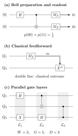
(a) Quantum wires carry an ordered register through $H$, controlled-NOT, and computational-basis measurements. (b) A measured classical record $m$ controls a later $X^m$ operation; this is different from coherent quantum control. (c) Width, gate count, and depth depend on the chosen gate and parallelism model.

Pure, Mixed, and Dynamic Circuits

Ideal unitary circuit

For a closed circuit with input state $\rho_{\mathrm{in}}$, the final state before measurement is

$$\rho_{\mathrm{final}} = U_C\rho_{\mathrm{in}}U_C^\dagger.$$

If an output register $O$ is measured in the computational basis and all other retained systems are denoted $R$, then

$$p(y) = \operatorname{Tr}\!\Big[ \big( \lvert y\rangle\langle y\rvert_O \otimes I_R \big) \times\rho_{\mathrm{final}} \Big].$$

The circuit outputs a sample from $p(y)$ unless the specification asks for a retained quantum state or an estimated expectation value. One run does not reveal every amplitude.

Channels, discard, and reset

A physical or generalized circuit may contain completely positive trace-preserving maps:

$$\mathcal E_C = \mathcal E_L \circ\cdots\circ \mathcal E_2 \circ \mathcal E_1.$$

Unitary gates are the special channels

$$\mathcal U(\rho) = U\rho U^\dagger.$$

Preparation, noise, reset, and discarding are naturally channels. Composing fixed maps on the displayed register assumes that each map describes that stage with the information retained so far. If an environment carries memory between stages, include that memory in the state or use a multi-time process description; independently fitted reduced channels need not compose correctly. A circuit that includes them need not have one unitary description on the displayed wires, although a larger unitary dilation may exist after adding environments and ancillas.

Measurements and records

A measurement instrument has completely positive, trace-nonincreasing outcome maps $\{\mathcal I_m\}$ whose sum is trace preserving. For input $\rho$,

$$p(m) = \operatorname{Tr} \mathcal I_m(\rho),$$

and, when $p(m)>0$,

$$\rho_m = \frac{ \mathcal I_m(\rho) }{ p(m) }.$$

If the record is retained, the output is a classical–quantum state:

$$\omega_{MQ} = \sum_m \lvert m\rangle\langle m\rvert_M \otimes \mathcal I_m(\rho).$$

The branch maps are generally trace nonincreasing. Their traces are probabilities, so normalizing every branch before recording those probabilities loses part of the circuit semantics.

Quantum Control and Classical Control

A coherently controlled unitary is itself a unitary gate:

$$C(U) = \lvert0\rangle\langle0\rvert \otimes I + \lvert1\rangle\langle1\rvert \otimes U.$$

The control wire may be in a superposition and can become entangled with the target. No classical outcome exists merely because the diagram contains a control dot.

Classical control is different. A measurement first produces a record $m$, and a later channel $\mathcal E_m$ is selected from that record. If the record is retained,

$$\omega_{MQ}' = \sum_m \lvert m\rangle\langle m\rvert_M \otimes \mathcal E_m\!\left( \mathcal I_m(\rho) \right).$$

If it is forgotten, sum over $m$. The resulting map can be irreversible even when every conditional $\mathcal E_m$ is unitary.

Under suitable conditions, a measurement used only to control later gates can be deferred by replacing classical control with coherent control and measuring later. This deferred-measurement principle is a model equivalence, not a claim that real-time measurement has no cost. Deferral may require extra coherent ancillas, change connectivity and depth, remove useful resets, or alter the physical noise exposure.

Measurement in circuits develops the basis rotations and readout rules. Mid-circuit measurement and feedforward treats causal branching, reset, reuse and the conditions for deferred measurement.

Input Conventions

The same diagram can answer different questions depending on its input: Common forms include:

• Fixed input: all data and ancillas begin in $\lvert0\rangle$.
• Classical input: a bitstring $x$ is encoded as $\lvert x\rangle$ or used to select gates.
• Quantum input: an arbitrary state $\rho_Q$ enters a named register, possibly entangled with an inaccessible reference $R$.
• Oracle access: a callable operation supplies information about a function or physical model. Its allowed inputs and permitted forward, inverse or controlled uses must be specified; see quantum oracles.
• Sample input: classical data are drawn from a stated distribution and encoded by a preparation procedure whose cost may matter.
• Advice or resource state: a state is supplied externally. Its preparation cost matters unless the model explicitly supplies it for free. For example, measurement-based computation consumes an entangled resource state. In complexity theory, advice can be nonuniform: it depends on input length without an efficient preparation rule.

Ancillas should be named and initialized. Assuming an unlimited supply of clean ancillas can change width, depth, reversibility, and fault-tolerance costs.

Output and Success Conventions

The output may be:

• a classical bit or bitstring;
• a sample from a target distribution;
• an estimate of an expectation value after many shots;
• a retained quantum state or channel;
• a success flag plus a conditional state;
• an accepted or rejected decision with bounded error.

For a classical input $x$ and output $y$, write the induced conditional distribution as

$$p_C(y\mid x).$$

For a postselected circuit, report both

$$p_{\mathrm{succ}} \quad\text{and}\quad \rho_{\mathrm{out}\mid\mathrm{succ}}.$$

A high conditional fidelity with exponentially small success probability is not a high-rate algorithm.

Circuit equivalence also depends on the output contract. Two closed circuits may implement the same unitary up to global phase. Two open circuits may implement the same channel. Two sampling circuits may have the same measured distribution while producing different unmeasured states. State which equivalence is relevant.

Width, Size, Depth, and Other Resources

Resource counts are meaningful only relative to a gate library and execution model.

Resource	Operational definition	Important dependence
Width	Maximum number of simultaneously live quantum wires	Includes data, ancillas, routing, syndrome, and workspace qubits
Gate count or size	Number of elementary gates	Depends on the declared gate set and approximation tolerance
Depth	Minimum number of allowed parallel layers respecting dependencies	Depends on connectivity, parallelism, and scheduling assumptions
Two-qubit gate count	Number of elementary gates acting on two qubits	Includes nonentangling gates such as SWAP if they are elementary; an entangling-gate count is a different convention
Query count	Calls to a specified oracle	Does not include ordinary gates unless stated
Measurement rounds	Sequential layers of measurement and feedforward	Depends on classical latency and adaptivity
$T$ count and $T$ depth	Non-Clifford resources in a fault-tolerant decomposition	Depends on code, synthesis target, and available resource states
Shot count	Repeated circuit executions used for statistical estimation	Depends on variance, confidence, mitigation, and grouping

If the elementary gates can be partitioned into layers $\mathcal L_1,\ldots,\mathcal L_D$ whose gates have disjoint supports, then

$$U_C = L_D\cdots L_2L_1,$$

with

$$L_\ell = \prod_{G\in\mathcal L_\ell}G.$$

This schedule has depth $D$; the minimum depth requires minimizing over all allowed schedules of the specified operations. Hardware routing can add SWAPs; calibration can prohibit simultaneous gates; measurement and feedforward can introduce latency; fault-tolerant protocols can replace one logical gate with a large spacetime structure. A circuit depth quoted without those assumptions is not a wall-clock runtime.

Circuit Families and Uniformity

One finite circuit can act on every input of its fixed register size. To handle arbitrarily growing input sizes, an algorithm is usually specified by a family

$$\{C_n\}_{n\geq1}$$

indexed by input size. The family is uniform when a classical procedure generates the description of $C_n$ efficiently from $1^n$. Uniformity prevents exponentially complicated answers from being hidden in an unexplained circuit description.

Complexity claims also need:

1. a fixed finite or efficiently describable gate set;
2. bounded gate locality;
3. an approximation metric and tolerance;
4. efficient classical descriptions of gate parameters;
5. a clear oracle or advice model.

Counting an arbitrary $2^n\times2^n$ unitary as one gate is formally a circuit but not an informative computational model. Its matrix requires exponentially many parameters in general.

Adiabatic computation provides a Hamiltonian-based model with polynomial equivalence to circuits under suitable uniformity, locality, norm and precision assumptions.

Worked Example: Preparing and Measuring a Bell Pair

Use register order $Q_1\otimes Q_2$ and input

$$\lvert\psi_0\rangle = \lvert00\rangle.$$

Apply $H$ to $Q_1$:

$$\begin{aligned} \lvert\psi_1\rangle &= (H\otimes I)\lvert00\rangle \\ &= \frac{ \lvert00\rangle+\lvert10\rangle }{\sqrt2}. \end{aligned}$$

Then apply controlled-NOT with $Q_1$ as control and $Q_2$ as target:

$$\begin{aligned} \lvert\psi_2\rangle &= \operatorname{CNOT}_{1\to2} \lvert\psi_1\rangle \\ &= \frac{ \lvert00\rangle+\lvert11\rangle }{\sqrt2} \\ &= \lvert\Phi^+\rangle. \end{aligned}$$

Thus the circuit unitary is

$$U_C = \operatorname{CNOT}_{1\to2} (H\otimes I).$$

Computational-basis measurement gives

$$\begin{gathered} p(00)=p(11)=\frac12, \\ p(01)=p(10)=0. \end{gathered}$$

The joint state contains coherence between $|00\rangle$ and $|11\rangle$, not just the classical correlation visible in this measurement. Measurements in other bases can test that distinction. Under the elementary gate set $\{H,\operatorname{CNOT}\}$, the preparation has width $2$, gate count $2$, and depth $2$. The two terminal measurements can occur in one measurement layer.

Circuit Model versus Hardware Execution

An abstract circuit is neither a pulse schedule nor a device schematic.

• A logical circuit specifies ideal operations on abstract or encoded systems.
• A compiled circuit rewrites those operations into a target gate set and connectivity graph.
• A scheduled circuit assigns compatible operations to time intervals.
• A control program produces pulses, voltages, optical fields, and readout decisions.
• A physical execution realizes noisy channels whose parameters drift and must be estimated.

These layers should not be collapsed when reporting depth, fidelity, runtime, or resource advantage. One logical controlled-NOT may be native on one platform, compiled from several interactions on another, or implemented fault tolerantly by code deformation, lattice surgery, teleportation, or magic-state-assisted gadgets. Hardware overview compares physical implementations.

Correctness and Error Metrics

The correct comparison depends on the output object.

• Compare pure output states up to global phase.
• Use trace distance or fidelity for states, with conventions stated.
• Use a channel metric such as diamond distance for worst-case process error.
• Use total variation distance for classical output distributions.
• Use an explicit failure probability for bounded-error decision or postselected circuits.
• Use an application-level observable error when that is the promised output.

Average gate fidelity alone does not determine a long circuit’s output error. Coherent errors can accumulate, correlations can invalidate independent-noise estimates, and postselection can hide failure probability. Noise in Quantum Information develops the practical taxonomy and diagnostic consequences. The Fidelity and Trace Distance entries provide compact state formulas; general channel theory remains in the open-systems volume.

Quantum channels for information processing explains how to model noisy operations. Error correction and fault tolerance addresses how a circuit can remain reliable when these operations are imperfect. For implementing the circuit, continue to gate decomposition, mapping and routing, or circuit simulation.

Exercises

1. Embedding gates into an ordered register. Use the convention

$$\lvert q_1q_2q_3\rangle = \lvert q_1\rangle \otimes\lvert q_2\rangle \otimes\lvert q_3\rangle.$$

Write the operator that applies $X$ to $Q_2$, and evaluate it on $\lvert010\rangle$. Then evaluate a controlled-NOT from $Q_1$ to $Q_3$ on $\lvert100\rangle$.

Solution

The embedded one-qubit gate is

$$X^{(2)} = I\otimes X\otimes I.$$

It flips only the middle factor:

$$(I\otimes X\otimes I) \lvert010\rangle = \lvert000\rangle.$$

For $\operatorname{CNOT}_{1\to3}$, the first qubit is the control and the third is the target. Because the control value in $\lvert100\rangle$ is $1$,

$$\operatorname{CNOT}_{1\to3} \lvert100\rangle = \lvert101\rangle.$$

Neither calculation can be inferred safely from an integer label unless the bit and tensor orders have first been declared.

2. Diagram order versus operator order. A one-qubit circuit applies $H$ and then $Z$ from left to right to input $\lvert0\rangle$. Find the final state. What state results if the matrix product is reversed by mistake?

Solution

The first gate is $H$, so the correct circuit unitary is

$$U_C=ZH.$$

Therefore

$$\begin{aligned} ZH\lvert0\rangle &= Z\lvert+\rangle \\ &= \lvert-\rangle. \end{aligned}$$

The mistaken product is $HZ$. Since $Z\lvert0\rangle=\lvert0\rangle$,

$$HZ\lvert0\rangle = H\lvert0\rangle = \lvert+\rangle.$$

The two states have the same computational-basis probabilities but opposite $X$-basis outcomes, so the ordering error is physically observable.

3. Bell-circuit output. Starting from $\lvert00\rangle$, apply $H$ to the first qubit and then $\operatorname{CNOT}_{1\to2}$. Compute the final density operator, both one-qubit reduced states, and the computational-basis output distribution.

Solution

The state-vector calculation gives

$$\lvert\Phi^+\rangle = \frac{ \lvert00\rangle+\lvert11\rangle }{\sqrt2}.$$

The density operator is

$$\rho_{\Phi^+} = \frac12\big( \lvert00\rangle\langle00\rvert + \lvert00\rangle\langle11\rvert + \lvert11\rangle\langle00\rvert + \lvert11\rangle\langle11\rvert \big).$$

Tracing out either subsystem removes the coherence terms and gives

$$\rho_1=\rho_2=\frac{I_2}{2}.$$

Terminal computational-basis measurement gives

$$\begin{gathered} p(00)=p(11)=\frac12, \\ p(01)=p(10)=0. \end{gathered}$$

Each local result is random, while the joint results are perfectly correlated.

4. Gate count and parallel depth. A three-qubit circuit has five gates with these dependencies:

• $H_1$ and $X_3$ have no predecessors;
• $\operatorname{CNOT}_{1\to2}$ follows $H_1$;
• $H_3$ follows $X_3$;
• $\operatorname{CZ}_{2,3}$ follows both $\operatorname{CNOT}_{1\to2}$ and $H_3$.

Find the gate count, width, and minimum ideal depth when gates on disjoint supports may run in parallel.

Solution

There are five elementary gates and three live wires, so

$$G=5, \qquad W=3.$$

A valid schedule is

$$\begin{aligned} \mathcal L_1 &= \{H_1,X_3\}, \\ \mathcal L_2 &= \{\operatorname{CNOT}_{1\to2},H_3\}, \\ \mathcal L_3 &= \{\operatorname{CZ}_{2,3}\}. \end{aligned}$$

The gates within each of the first two layers act on disjoint supports. The final controlled-$Z$ must wait for both predecessor branches, so no two-layer schedule satisfies the dependencies. Hence

$$D=3.$$

Connectivity or calibration constraints could increase the physical depth.

5. Why a CNOT is not a cloning branch. Let

$$\lvert\psi\rangle = \alpha\lvert0\rangle + \beta\lvert1\rangle.$$

Apply a controlled-NOT to $\lvert\psi\rangle\otimes\lvert0\rangle$. Compare the result with $\lvert\psi\rangle\otimes\lvert\psi\rangle$.

Solution

Linearity gives

$$\operatorname{CNOT} \left( \lvert\psi\rangle\otimes\lvert0\rangle \right) = \alpha\lvert00\rangle + \beta\lvert11\rangle.$$

A true clone would be

$$\lvert\psi\rangle^{\otimes2} =\; \alpha^2\lvert00\rangle + \alpha\beta\lvert01\rangle + \alpha\beta\lvert10\rangle + \beta^2\lvert11\rangle.$$

These states are unequal for a generic superposition. The controlled-NOT copies the computational-basis label when the input is $\lvert0\rangle$ or $\lvert1\rangle$; on a superposition it generally creates entanglement. A branching wire would incorrectly assert universal cloning.

6. Measurement-based active reset. Measure one qubit in the computational basis, obtaining $m\in\{0,1\}$, and then apply $X^m$. Show that the unconditioned output is $\lvert0\rangle\langle0\rvert$ for every input density operator $\rho$. What information remains in the classical record?

Solution

Let

$$P_0=\lvert0\rangle\langle0\rvert, \qquad P_1=\lvert1\rangle\langle1\rvert.$$

The unnormalized measurement branches are $P_m\rho P_m$. After the conditional corrections,

$$\begin{aligned} \widetilde\rho_0' &= P_0\rho P_0 = \rho_{00}\lvert0\rangle\langle0\rvert, \\ \widetilde\rho_1' &= X P_1\rho P_1 X = \rho_{11}\lvert0\rangle\langle0\rvert. \end{aligned}$$

Forgetting the record gives

$$\begin{aligned} \rho' &= \widetilde\rho_0' + \widetilde\rho_1' \\ &= (\rho_{00}+\rho_{11}) \lvert0\rangle\langle0\rvert \\ &= \lvert0\rangle\langle0\rvert. \end{aligned}$$

The retained classical record has probabilities

$$p(0)=\rho_{00}, \qquad p(1)=\rho_{11}.$$

It remembers the measured computational-basis population even though the corrected quantum output is always reset. The input coherence is destroyed, so this displayed-wire operation is not unitary. If the input qubit was correlated with an inaccessible reference $R$, the unconditioned result is $|0\rangle\langle0|\otimes\rho_R$. For a Bell input, the recorded bit remains classically correlated with $R$, even though the reset qubit is now uncorrelated with both. Resetting a local wire does not reconstruct its previous joint quantum state.

References

• D. Aharonov, A. Kitaev, and N. Nisan, “Quantum Circuits with Mixed States”, Proceedings of the 30th Annual ACM Symposium on Theory of Computing, 20–30 (1998).
• A. Barenco, C. H. Bennett, R. Cleve, D. P. DiVincenzo, N. Margolus, P. Shor, T. Sleator, J. A. Smolin and H. Weinfurter, “Elementary Gates for Quantum Computation”, Physical Review A 52, 3457–3467 (1995).
• E. Bernstein and U. Vazirani, “Quantum Complexity Theory”, SIAM Journal on Computing 26, 1411–1473 (1997).
• D. Deutsch, “Quantum Computational Networks”, Proceedings of the Royal Society A 425, 73–90 (1989).
• R. B. Griffiths and C.-S. Niu, “Semiclassical Fourier Transform for Quantum Computation”, Physical Review Letters 76, 3228–3231 (1996).
• A. Yu. Kitaev, A. H. Shen, and M. N. Vyalyi, Classical and Quantum Computation, American Mathematical Society (2002).
• N. D. Mermin, Quantum Computer Science: An Introduction, Cambridge University Press (2007).
• M. A. Nielsen and I. L. Chuang, Quantum Computation and Quantum Information, 10th anniversary ed., Cambridge University Press (2010).
• J. Preskill, Lecture Notes for Physics 219/Computer Science 219: Quantum Computation, Caltech, living course notes.
• J. Watrous, The Theory of Quantum Information, Cambridge University Press (2018).
• A. C.-C. Yao, “Quantum Circuit Complexity”, Proceedings of the 34th Annual Symposium on Foundations of Computer Science, 352–361 (1993).