Mid-Circuit Measurement and Feedforward

An adaptive quantum circuit is a quantum–classical execution process: a measurement produces a classical record, and that record can change which operation, measurement, or stopping rule is used later. An outcome probability alone therefore does not define the circuit. The full object includes the state on every branch, the causal availability of records, the types and lifetimes of branch outputs, and the rule for combining terminal histories.

We will follow finite circuits branch by branch, calculate reset and correction maps, and compare average costs with the longest possible execution. The numerical timing examples are hypothetical schedules, not measurements of a device.

Helpful background. Measurement in circuits introduces subnormalized outcome maps, classical records and the distinction between selected and unread states.

Dynamic Quantum–Classical Circuits

A static unitary circuit denotes one linear operator, while a dynamic circuit denotes a causal family of quantum operations indexed by classical histories. If $h=m_1m_2\cdots m_k$ is the record available at one point in an execution, then a later instrument, channel, or stop decision may depend on $h$. The history is data, not a coherent quantum label unless the circuit explicitly stores it in a quantum register.

Three objects must be kept distinct:

• a coherent controlled operation applies different target blocks while retaining off-diagonal control coherences;
• measurement-conditioned feedforward creates a classical record and then chooses a later channel from that record;
• postprocessing acts on data after the quantum job has ended and cannot change the already completed quantum evolution.

The first two can agree on a basis-state truth table while defining different channels on superpositions. Controlled Operations explains the coherent block-unitary case. Here the relevant object is a measured, classically indexed process.

Specify what the circuit returns. It may return a final quantum register, the full classical history, a coarsened success flag, a history-conditioned state, or only an unconditional mixture. Forgetting a history is a classical marginalization and a quantum mixture; it is never an amplitude sum over alternatives.

Instruments, Conditional Channels, and History Probabilities

Let $h$ label a classical history at an internal node and $m$ the next reported outcome. Let $\mathcal I_m^{(h)}$ be the outcome map chosen at that node, and let $\mathcal C_{hm}$ be the subsequent conditional channel. Starting with $\widetilde{\rho}_{\emptyset}=\rho$, define

$$\begin{aligned} \widetilde{\rho}_{hm} &= (\mathcal C_{hm}\circ\mathcal I_m^{(h)})(\widetilde{\rho}_h) \\ &= \mathcal C_{hm}(\mathcal I_m^{(h)}(\widetilde{\rho}_h)), \\ p(hm) &= \operatorname{Tr}\widetilde{\rho}_{hm}. \end{aligned}$$

The trace is the joint probability of the complete history $hm$, not merely a probability conditional on reaching $h$. When $p(h)>0$,

$$p(m\mid h) = \frac{p(hm)}{p(h)}, \qquad \rho_{hm} = \frac{\widetilde{\rho}_{hm}}{p(hm)} \quad (p(hm)>0).$$

At each reachable node, the instrument is complete and every subsequent conditional channel preserves trace. Include loss or abort explicitly among the recorded outcomes, with a suitable flag state if no qubit survives; an unexplained trace decrease would omit some executions. A zero-probability branch has a zero subnormalized state; it has no normalized posterior that can be used in a later calculation.

Let $\mathcal L$ be a prefix-free set of terminal histories. Equivalently, one may compare all histories at one fixed depth, padding branches that have already terminated. If the classical history register $H$ encodes termination and record length, the final classical-quantum state and its history-forgotten quantum output are, assuming all returned quantum states have been placed in the same output space $Q$,

$$\Omega_{HQ} = \sum_{h\in\mathcal L} |h\rangle\langle h|_H \otimes \widetilde{\rho}_h,$$ $$\rho_{\mathrm{out}} = \operatorname{Tr}_H\Omega_{HQ} = \sum_{h\in\mathcal L}\widetilde{\rho}_h.$$

A complete capped policy satisfies

$$\sum_{h\in\mathcal L} \operatorname{Tr}\widetilde{\rho}_h =1.$$

Never sum both an internal history and any of its descendants. That double counts executions. A prefix-free set must also cover every possible exit: $\{0,10\}$ would omit history $11$. A complete terminal set such as $\{0,10,11\}$ is valid because no member is a prefix of another; the set $\{1,10,11\}$ is not.

Classical Predicates, Dataflow, and Branch Merges

A predicate may depend only on records that exist at that point in the causal schedule. For example, the rule “apply $X$ when $m=1$” presupposes a reported bit $m$, a declared encoding of detector outcomes into that bit, and a path by which the bit reaches the conditional operation. Branching on an unobserved ideal detector variable while the controller receives a noisy reported code describes a different process.

At a branch merge, a later quantum operation must have a qubit to act on in every incoming branch. If one branch discards $q$ and another retains it, either return only classical data from both branches or explicitly prepare a replacement where needed. If the branches carry different Pauli corrections, keep the correction label with the qubit so later gates and measurements can interpret it consistently.

Circuit intermediate representations describes how programming languages represent this control flow.

Reset, Release, and Qubit Reuse

Reset is a channel with a declared postcondition. It is not an inverse of measurement and need not restore coherence with any system that was correlated with the measured qubit. For computational-basis measurement with $P_m=|m\rangle\langle m|$, measurement followed by $X^m$ gives

$$\begin{aligned} \mathcal R(\rho) &= \sum_{m=0}^1 X^mP_m\rho P_mX^m \\ &= |0\rangle\langle0|\operatorname{Tr}\rho. \end{aligned}$$

This channel sends every normalized input to $|0\rangle\langle0|$. It removes the input coherence and is many-to-one, so it is neither unitary nor invertible. If the bit $m$ was copied into a classical register, that record still contains the outcome distribution after the quantum reset.

Reset prepares a specified state; releasing a qubit means that the program will no longer use it; reuse assigns it a new task after any needed preparation. Reusing the same wire label does not restore a destructively measured system. Physical reset can also have errors or leakage that are absent from the ideal channel above.

Physical Corrections and Pauli-Frame Updates

A physical correction applies a quantum operation. A Pauli-frame update instead stores a classical description of an outstanding Pauli and changes how later gates or measurements are interpreted. The two methods can implement the same logical output only if every later operation consumes the frame consistently.

Define the frame by $\rho_{\rm physical}=F\rho_{\rm logical}F^\dagger$. Write a one-qubit frame, up to phase, as

$$F(a,b)=X^aZ^b, \qquad a,b\in\{0,1\}.$$

If the next physical gates are $H$ and then $S$, conjugation gives

$$S H F(a,b) H^\dagger S^\dagger \doteq X^bZ^{a\oplus b},$$

where $\doteq$ denotes equality up to a global phase. A later physical $Z$-basis measurement is flipped by the $X$ exponent of the propagated frame, so, writing $z$ for the recorded bit rather than the eigenvalue $(-1)^z$,

$$z_{\mathrm{logical}} = z_{\mathrm{physical}}\oplus b.$$

The frame must therefore remain associated with its branch. Merging two quantum values while discarding different outstanding frames generally corrupts later predictions. Across Clifford gates a Pauli frame remains Pauli, but across a non-Clifford gate it may not. Blindly updating two bits by XOR is then invalid; the circuit must change the correction strategy, adapt a later measurement, or enlarge the tracked object.

Deferred Measurement and Its Failure Conditions

The deferred-measurement principle compares specified final outputs; intermediate processes can still differ. In its familiar finite form, a measurement whose result only selects a later unitary can sometimes be replaced by coherent control, with the control measured at the end. The replacement must reproduce the declared final quantum state and classical record. A common phase multiplying one finally measured branch cancels from its outcome map; phases within a branch that affect interference must be preserved.

For this simple replacement to work:

• the removed record is not read, reported, or used by a host before the new terminal measurement;
• the would-be control system remains available and is not destructively measured, reset, released, or reused;
• no intervening noncommuting operation uses coherence that one formulation removes and the other retains;
• coherent controlled access to the required branch operation is part of the declared interface;
• the equivalence is claimed only for the compared outputs, not for latency, detector behavior, noise, or physical resource cost.

Early termination, repeated measurement, invalid-code handling, and a timeout can make a dynamic policy impossible to replace by a single deferred meter without adding further coherent storage and control. Even when the final ideal statistics agree, the physical implementations can have different exposure to noise and different timing constraints.

Measurement in Circuits proves the elementary deferred-CNOT example. The semiclassical Fourier-transform construction of Griffiths and Niu is an important positive example of feedforward, but it is not a blanket theorem that all adaptive measurements can be deferred.

Latency, Deadlines, and Branch-Aware Resources

Timing claims require absolute events as well as durations. For a history $h$, let $t_{\mathrm{record}}(h)$ be a specified event time before the reported-record processing path begins. Let $L_{\mathrm{ff}}(h)$ include the declared acquisition, classification, decision, and dispatch path not already included in that event time, and let $t_{\mathrm{branch}}(h)$ be the duration of the conditional branch operation. Then

$$\begin{aligned} t_{\mathrm{ready}}(h) &= t_{\mathrm{record}}(h) +L_{\mathrm{ff}}(h) +t_{\mathrm{branch}}(h), \\ s_{\mathrm{raw}}(h) &= t_{\mathrm{deadline}}(h) -t_{\mathrm{ready}}(h). \end{aligned}$$

If the declared jitter or safety guard is $g(h)\geq0$, the residual slack is

$$s_{\mathrm{guarded}}(h) = s_{\mathrm{raw}}(h)-g(h).$$

A complete schedule passes only if the minimum guarded slack over the relevant terminal branches is nonnegative. A mean latency cannot establish this result: a rare branch can miss a coherence-sensitive deadline even when the average branch is fast.

Resources in an adaptive circuit are random variables on terminal histories. For a resource count or duration $R$,

$$\mathbb E[R] = \sum_{h\in\mathcal L}p(h)R(h), \qquad R_{\max} = \max_{h\in\mathcal L}R(h).$$

If a result is conditioned on success, use renormalized success-leaf weights and report the success probability separately. Measurement count, conditional gate count, quantum width, live classical memory, elapsed time, abstract query count, and physical duration measure different resources. They should not be collapsed into one unlabeled “cost.”

A fixed guard gives a hard deadline guarantee only if it bounds the possible extra delay. If it is instead chosen from a jitter quantile, the schedule has the corresponding probabilistic timing guarantee. Control, readout and calibration discusses physical acquisition paths and controller behavior.

Worked example: active reset and reuse

Take a qubit in

$$\rho=\begin{pmatrix}2/3&1/6\\1/6&1/3\end{pmatrix}, \qquad \operatorname{Tr}\rho^2=\frac{11}{18}.$$

A computational Lüders measurement gives probabilities $p_0=2/3,p_1=1/3$. Apply $X$ only after outcome one. The two corrected, subnormalized branches are

$$\widetilde\rho_0=\frac23|0\rangle\langle0|, \qquad \widetilde\rho_1=\frac13|0\rangle\langle0|.$$

Consequently the reset output is pure, while the retained classical bit is still random:

$$\Omega_{MQ}=\operatorname{diag}(2/3,1/3)_M\otimes|0\rangle\langle0|_Q.$$

Its record entropy is $h_2(1/3)\simeq0.918296$ bits. Resetting the qubit has not erased the measurement record.

For a simple reuse test, apply $H$ and then measure $X$. Correct reset gives the $+$ outcome with certainty. Omitting the conditional flip leaves $\operatorname{diag}(2/3,1/3)$ before $H$, so the same test gives $p(+)=2/3$. The two output distributions have total variation distance $1/3$.

Suppose measurement ends at $240\,\mathrm{ns}$, the subsequent record path takes $100\,\mathrm{ns}$, and the conditional flip takes $20\,\mathrm{ns}$. The longest branch completes at $360\,\mathrm{ns}$. A $400\,\mathrm{ns}$ deadline leaves $40\,\mathrm{ns}$, or $15\,\mathrm{ns}$ after a $25\,\mathrm{ns}$ guard. Every execution uses one measurement; the expected number of flips is $1/3$ and the maximum is one.

Worked example: at most two attempts

Start in $|+\rangle$ and measure $Z$, accepting outcome zero as success. After a first outcome one, apply $X$ and then $H$ to prepare a fresh $|+\rangle$ and try once more. After a second failure, apply $X$ to reset the qubit and report exhaustion. The terminal histories are

$$p(0)=\frac12,\qquad p(10)=\frac14,\qquad p(11)=\frac14.$$

Success has probability $3/4$ and exhaustion probability $1/4$. Conditioned on success, histories $0$ and $10$ have weights $2/3$ and $1/3$. All three final qubit states are $|0\rangle$, so the quantum state alone does not reveal whether the policy succeeded. Keep the success flag or the history when that distinction matters.

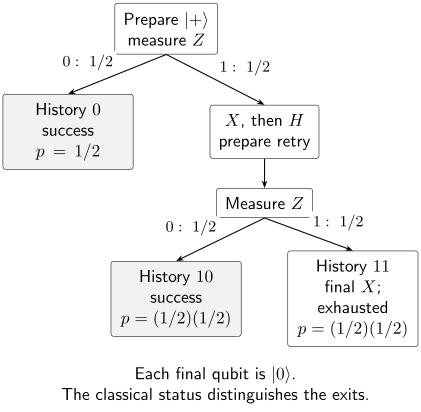
Only the terminal histories are summed. The probability of reaching the second measurement is $1/2$, and its two conditional outcomes are each equally likely. Including the internal history $1$ as well as its descendants would count those executions twice.

Use the following hypothetical timing: first measurement ends at $200\,\mathrm{ns}$, followed by an $80\,\mathrm{ns}$ report path. On failure, $X$ and $H$ take $20\,\mathrm{ns}$ each. The second measurement then runs from $320$ to $520\,\mathrm{ns}$, with its report ready at $600\,\mathrm{ns}$. A final failure correction ends at $620\,\mathrm{ns}$.

History	Probability	Measurements	$X$ gates	Retry $H$ gates	End time (ns)
$0$	$1/2$	1	0	0	280
$10$	$1/4$	2	1	1	600
$11$	$1/4$	2	2	1	620

Weighting each row gives

$$\begin{aligned} \mathbb E[N_{\rm meas}]&=3/2,&N_{{\rm meas},\max}&=2,\\ \mathbb E[N_X]&=3/4,&\mathbb E[N_{H,\rm retry}]&=1/2,\\ \mathbb E[T]&=445\,\mathrm{ns},&T_{\max}&=620\,\mathrm{ns}. \end{aligned}$$

A $650\,\mathrm{ns}$ deadline with zero additional guard leaves only $30\,\mathrm{ns}$ on the longest branch, even though the mean time is much shorter. The fair-attempt calculation relies on the explicit reset and re-preparation. In a general quantum repeat-until-success protocol, a failed attempt may disturb an unknown input; the failure map must be analyzed before assuming independent retries.

When retries measure the input

The preceding preparation example can recreate its known input. To see what changes for an unknown input, consider a two-outcome instrument on the same qubit at every attempt:

$$K_s=\begin{pmatrix}\sqrt{1-q_0}&0\\0&\sqrt{1-q_1}\end{pmatrix}, \qquad K_f=\begin{pmatrix}\sqrt{q_0}&0\\0&\sqrt{q_1}\end{pmatrix}, \qquad 0\le q_0,q_1<1.$$

They obey $K_s^\dagger K_s+K_f^\dagger K_f=I$. Here “success” means only the reported label $s$; no target gate is presumed. After $f$, apply the same instrument again without a correction or re-preparation, stopping at the first $s$. The branch operator for stopping on attempt $k$ is $A_k=K_sK_f^{k-1}$. For an input density matrix $\rho$, the survival probability and mean stopping time follow by summing the failure histories:

$$\begin{aligned} \Pr(N>n)&=\operatorname{Tr}\!\bigl(K_f^n\rho(K_f^n)^\dagger\bigr) =\rho_{00}q_0^n+\rho_{11}q_1^n,\\ \mathbb E[N]&=\sum_{n=0}^{\infty}\Pr(N>n) =\frac{\rho_{00}}{1-q_0}+\frac{\rho_{11}}{1-q_1}. \end{aligned}$$

For $|+\rangle$, $q_0=1/4$ and $q_1=3/4$, the first attempt succeeds with probability $1/2$. After one failure the populations are $1/4,3/4$, so the next conditional success probability is $3/8$. Consequently $\mathbb E[N]=8/3$, rather than $2$ from an unjustified fair-trial model. Termination occurs with probability one, but there is no finite worst-case attempt count in this example.

Eventual success also need not preserve the input. When the stopping record is forgotten, summing the successful branches gives

$$\mathcal E(\rho)=\sum_{k=1}^{\infty}A_k\rho A_k^\dagger =\begin{pmatrix}\rho_{00}&c\rho_{01}\\c\rho_{10}&\rho_{11}\end{pmatrix}, \qquad c=\frac{\sqrt{(1-q_0)(1-q_1)}}{1-\sqrt{q_0q_1}}.$$

The off-diagonal factor is the geometric sum of the two branch amplitudes; $c<1$ whenever $q_0\ne q_1$. The stopping time contains information about the computational-basis component. In the numerical example, $c=\sqrt3/(4-\sqrt3)\simeq0.763708$, and the output has squared fidelity $(1+c)/2\simeq0.881854$ with the initial $|+\rangle$, despite eventual reported success being certain.

A standard unitary repeat-until-success construction instead arranges $K_s=\sqrt p\,U$ and failure branches $K_{f,j}=\sqrt{p_j}\,V_j$, with known unitaries $V_j$ whose inverses are applied before retrying, $0<p\le1$, and $p+\sum_jp_j=1$. Each corrected failure restores the unknown input, including its correlations with a reference, so the success probability stays $p$ and the mean attempt count is $1/p$. Recovery operations still contribute to physical cost. Paetznick and Svore give this construction; the general instrument description explains why a failure probability alone cannot establish it.

Exercises

Exercise 1: One Measurement-Conditioned Channel

For

$$\rho = \begin{pmatrix} 1/2&1/4\\ 1/4&1/2 \end{pmatrix},$$

perform an $X$-basis Lüders measurement, encode $+\mapsto0$ and $-\mapsto1$, and apply $Z^m$. Find the outcome probabilities, corrected conditional outputs, cq state in $M\otimes Q$ order, and history-forgotten output.

Solution

With $P_\pm=|\pm\rangle\langle\pm|$,

$$p_+ = \langle+|\rho|+\rangle = \frac34, \qquad p_- = \frac14.$$

The uncorrected branches are $(3/4)P_+$ and $(1/4)P_-$. Since $Z|-\rangle=|+\rangle$, applying $Z^m$ gives

$$\widetilde\rho_0' = \frac34P_+, \qquad \widetilde\rho_1' = \frac14P_+.$$

Both normalized conditional outputs are $|+\rangle$. Therefore

$$\Omega_{MQ} = \left( \frac34|0\rangle\langle0|_M + \frac14|1\rangle\langle1|_M \right) \otimes P_+,$$

and forgetting $M$ gives $\rho_{\mathrm{out}}=P_+$.

Exercise 2: Normalize a Two-Stage Branch Tree

The first binary outcome is fair. Only after $m_1=1$, a second measurement has $p(m_2=0\mid m_1=1)=3/4$. A zero terminates successfully. Find the terminal probabilities for $0,10,11$, the success probability, the expected measurement count, and the success-conditioned history weights.

Solution

The prefix-free terminal probabilities are

$$p(0)=\frac12, \qquad p(10)=\frac12\frac34=\frac38, \qquad p(11)=\frac12\frac14=\frac18.$$

They sum to one. Histories $0$ and $10$ are successful, so

$$p(\text{success}) = \frac12+\frac38 = \frac78.$$

One measurement is used on history $0$ and two on histories $10$ and $11$:

$$\mathbb E[N_{\mathrm{meas}}] = \frac12(1) + \left(\frac38+\frac18\right)(2) = \frac32.$$

Conditioning the two successful leaves on their total probability $7/8$ gives

$$p(0\mid\text{success})=\frac47, \qquad p(10\mid\text{success})=\frac37.$$

Exercise 3: Prove the Active-Reset Channel

For

$$\rho = \begin{pmatrix} a&c\\ c^*&1-a \end{pmatrix},$$

prove that computational-basis measurement followed by $X^m$ produces $|0\rangle\langle0|$. Track the classical record and classify the resulting quantum channel.

Solution

The corrected branch Kraus operators may be written

$$K_0=P_0=|0\rangle\langle0|, \qquad K_1=XP_1=|0\rangle\langle1|.$$

They satisfy

$$K_0^\dagger K_0+K_1^\dagger K_1 = P_0+P_1 =I,$$

so the map is completely positive and trace preserving. Its output is

$$\begin{aligned} \mathcal R(\rho) &= K_0\rho K_0^\dagger + K_1\rho K_1^\dagger \\ &= aP_0+(1-a)P_0 = P_0. \end{aligned}$$

The record has probabilities $p(0)=a$ and $p(1)=1-a$; the coherence $c$ is absent from both recorded branches. The quantum channel is constant-output, CPTP, nonunitary, and noninvertible. Retaining the bit preserves the classical distribution even though the quantum marginal is always $P_0$.

Exercise 4: Propagate a Pauli Frame

An outstanding frame is $F=X^aZ^b$. Propagate it through physical $H$ followed by $S$, up to global phase. How must a final physical $Z$-measurement bit be interpreted?

Solution

First use $HXH=Z$ and $HZH=X$:

$$HFH \doteq X^bZ^a.$$

Then $SXS^\dagger\doteq XZ$ and $SZS^\dagger=Z$, so

$$S(HFH)S^\dagger \doteq X^bZ^{a\oplus b}.$$

The propagated $X$ exponent is $b$, and an $X$ flips a physical $Z$-measurement outcome. Hence

$$z_{\mathrm{logical}} = z_{\mathrm{physical}}\oplus b.$$

The answer is a classical reinterpretation only if the frame remains tracked; otherwise the outstanding correction must be applied physically.

Exercise 5: Repair an Ill-Typed Branch Merge

Branch $m=0$ returns $(m,q)$ with $q$ live. Branch $m=1$ destructively measures or releases $q$ and returns only $m$. Diagnose a later merged use of $q$ and give two valid repairs. What should be merged if both branches retain a qubit but carry different Pauli frames?

Solution

The merge is ill typed: one incoming edge supplies a live quantum value and the other does not. A later gate on a merged symbol $q$ therefore has no channel semantics on the $m=1$ branch.

One repair is to make both branches record-only and forbid later quantum use. A second is to prepare or reset an explicit replacement in branch $1$, then return a qubit in the specified output space on each branch, with its preparation and any outstanding correction identified. The replacement is a new declared value; reusing the old wire label does not undo destructive measurement or release.

If both qubits remain live but their Pauli frames differ, merge $(q,\mathrm{frame})$. Dropping the frame would make later gates and measurement interpretations branch dependent without recording that dependence.

Exercise 6: Compute Deadline Slack

A measurement interaction ends at $1000\,\mathrm{ns}$. The subsequent acquisition, classification, decision, and dispatch take $90,35,25,10\,\mathrm{ns}$. The dependent operation must start by $1200\,\mathrm{ns}$ and the declared guard is $20\,\mathrm{ns}$. Find the earliest start time, raw slack, and residual slack. No gate duration is included in this start-time deadline. Repeat if classification takes $65\,\mathrm{ns}$.

Solution

For the first schedule, the record path lasts

$$90+35+25+10 = 160\ \mathrm{ns},$$

so

$$t_{\mathrm{start}} = 1000+160 = 1160\ \mathrm{ns}.$$

The raw slack is $1200-1160=40\,\mathrm{ns}$, and subtracting the guard leaves $20\,\mathrm{ns}$. The guarded schedule passes.

Increasing classification from $35$ to $65\,\mathrm{ns}$ adds $30\,\mathrm{ns}$:

$$t_{\mathrm{start}}' = 1190\ \mathrm{ns}.$$

Raw slack is now $10\,\mathrm{ns}$ and residual slack is $10-20=-10\,\mathrm{ns}$. The guarded schedule fails even though the unguarded operation arrives before the deadline.

Exercise 7: Cap a Geometric Retry Policy

Independent attempts succeed with probability $0.3$. At most four attempts are allowed. Find the probability of success by the cap, the exhaustion probability, the expected number of attempts, and the worst-case count.

Solution

The failure probability per attempt is $q=0.7$. Four consecutive failures have probability

$$q^4 = 0.7^4 = 0.2401.$$

Therefore

$$p(\text{success by cap}) = 1-q^4 = 0.7599.$$

The exhaustion probability is $0.2401$. This policy has no separate abort or timeout exit, so both of those probabilities are zero.

Attempt $k$ is reached only after the first $k-1$ failures, so

$$\begin{aligned} \mathbb E[N] &= 1+q+q^2+q^3 \\ &= 1+0.7+0.49+0.343 \\ &= 2.533. \end{aligned}$$

The worst case is four attempts. A state or statistic conditioned on the $0.7599$ success event is postselected; the capped policy is not a deterministic transformation.

Exercise 8: Bell-branch correction

Prepare $|\Phi^+\rangle$ in the order $q_0q_1$. Measure $q_0$ in the $X$ basis, encoding $+\mapsto0$ and $-\mapsto1$. How can the result prepare logical $|+\rangle$ on $q_1$? Compare a physical correction, a tracked frame, and omission of both.

Solution

The identity

$$|\Phi^+\rangle=\frac{|+\rangle|+\rangle+|-\rangle|-\rangle}{\sqrt2}$$

shows that the two outcomes are equally likely and leave $q_1$ in $|+\rangle$ or $|-\rangle$. Physical $Z^m$ maps both to $|+\rangle$. After discarding $q_0$, the corrected classical–quantum state is

$$\Omega_{MQ_1}=\frac{I_M}{2}\otimes|+\rangle\langle+|.$$

Alternatively, keep the physical $|-\rangle$ on branch one and record a $Z$ frame. A later physical $X$-measurement bit must be flipped on that branch. The logical outcome is then the same, though no corrective pulse was applied.

If both the correction and its frame are omitted and the outcome is forgotten, the output is $I/2$. Its squared fidelity with $|+\rangle$ is $1/2$ and its trace distance is $1/2$; its $X$ expectation is zero instead of one.

For an illustrative timing check, a measurement ending at $100\,\mathrm{ns}$, a $40\,\mathrm{ns}$ report path and a $20\,\mathrm{ns}$ correction give a longest completion time of $160\,\mathrm{ns}$. A $180\,\mathrm{ns}$ deadline leaves $20\,\mathrm{ns}$ before any extra guard. The expected physical $Z$ count is $1/2$; the frame version has a different classical processing requirement.

Exercise 9: Keep the exhaustion branch

Cap the preceding unknown-input instrument at two attempts. For $q_0=1/4,q_1=3/4$ and input $|+\rangle$, find the success and exhaustion probabilities and the computational-basis populations after exhaustion. Show that including exhaustion gives a trace-preserving instrument for every input.

Solution

The three terminal operators are $K_s$, $K_sK_f$, and $K_f^2$. Since the diagonal operators commute,

$$K_s^\dagger K_s+(K_sK_f)^\dagger(K_sK_f) +(K_f^2)^\dagger K_f^2=I.$$

Their probabilities on $|+\rangle$ are $1/2,3/16,5/16$, respectively. Thus success has probability $11/16$ and exhaustion $5/16$. The exhausted state is $(|0\rangle+3|1\rangle)/\sqrt{10}$, with populations $1/10,9/10$; the failed attempts have changed the unknown input. Dropping that branch leaves a trace-decreasing success operation. Normalizing it describes postselection, not the complete capped procedure.

References

• D. Aharonov, A. Kitaev, and N. Nisan, “Quantum Circuits with Mixed States,” Proceedings of the 30th Annual ACM Symposium on Theory of Computing, 20–30 (1998), doi:10.1145/276698.276708.
• E. Bäumer et al., “Efficient Long-Range Entanglement Using Dynamic Circuits,” PRX Quantum 5, 030339 (2024), doi:10.1103/PRXQuantum.5.030339.
• C. H. Bennett, G. Brassard, C. Crépeau, R. Jozsa, A. Peres, and W. K. Wootters, “Teleporting an Unknown Quantum State via Dual Classical and Einstein–Podolsky–Rosen Channels,” Physical Review Letters 70, 1895–1899 (1993), doi:10.1103/PhysRevLett.70.1895.
• A. D. Córcoles et al., “Exploiting Dynamic Quantum Circuits in a Quantum Algorithm with Superconducting Qubits,” Physical Review Letters 127, 100501 (2021), doi:10.1103/PhysRevLett.127.100501.
• A. W. Cross et al., “OpenQASM 3: A Broader and Deeper Quantum Assembly Language,” ACM Transactions on Quantum Computing 3, article 12 (2022), doi:10.1145/3505636.
• D. Gottesman and I. L. Chuang, “Demonstrating the Viability of Universal Quantum Computation Using Teleportation and Single-Qubit Operations,” Nature 402, 390–393 (1999), doi:10.1038/46503.
• R. B. Griffiths and C.-S. Niu, “Semiclassical Fourier Transform for Quantum Computation,” Physical Review Letters 76, 3228–3231 (1996), doi:10.1103/PhysRevLett.76.3228.
• M. A. Nielsen and I. L. Chuang, Quantum Computation and Quantum Information, 10th Anniversary Edition, Cambridge University Press (2010), doi:10.1017/CBO9780511976667.
• A. Paetznick and K. M. Svore, “Repeat-Until-Success: Non-deterministic decomposition of single-qubit unitaries,” Quantum Information and Computation 14(15–16), 1277–1301 (2014), doi:10.26421/QIC14.15-16-2, arXiv:1311.1074.
• R. Raussendorf and H. J. Briegel, “A One-Way Quantum Computer,” Physical Review Letters 86, 5188–5191 (2001), doi:10.1103/PhysRevLett.86.5188.
• D. Ristè, C. C. Bultink, K. W. Lehnert, and L. DiCarlo, “Feedback Control of a Solid-State Qubit Using High-Fidelity Projective Measurement,” Physical Review Letters 109, 240502 (2012), doi:10.1103/PhysRevLett.109.240502.
• P. Selinger and B. Valiron, “A Lambda Calculus for Quantum Computation with Classical Control,” Mathematical Structures in Computer Science 16, 527–552 (2006), doi:10.1017/S0960129506005238.
• J. Watrous, The Theory of Quantum Information, Cambridge University Press (2018), doi:10.1017/9781316848142.