Continuous-Variable Quantum Computation

Continuous-variable quantum computation processes bosonic modes through their quadratures, using operations such as displacements, squeezing, mode coupling and measurement. Gaussian states and operations form a useful tractable sector: first and second moments describe the quantum state completely. Universal polynomial computation needs resources outside that sector, together with assumptions about available controls, energy and approximation accuracy.

A mode is an infinite-dimensional system, not an unlimited store of freely readable information. Real inputs have finite energy, measurements have finite resolution, and a numerical cutoff must be justified. Bosonic and encoded computation models instead studies finite logical systems encoded inside oscillators.

Helpful background. Continuous-variable systems introduces quadrature and Fock representations. Gaussian states and Wigner functions explains covariance matrices and the uncertainty condition.

Quadratures, energy and finite cutoffs

This page uses $\hbar=1$ and

$$[a_j,a_k^\dagger] = \delta_{jk}, \qquad q_j = \frac{a_j+a_j^\dagger}{\sqrt2}, \qquad p_j = \frac{a_j-a_j^\dagger}{i\sqrt2}.$$

Thus $[q_j,p_k]=i\delta_{jk}$ and the vacuum variances are $\operatorname{Var}(q_j)=\operatorname{Var}(p_j)=1/2$. A covariance quoted in a convention with vacuum variance $1/4$ or $1$ must be rescaled before it is combined with formulas here.

Order the quadratures of $m$ modes as

$$R = (q_1,p_1,\ldots,q_m,p_m)^{\mathsf T}, \qquad [R_j,R_k] = i\Omega_{jk},$$

with

$$\Omega = \bigoplus_{j=1}^{m} \begin{pmatrix} 0&1\\ -1&0 \end{pmatrix}.$$

The first moments and covariance are

$$d = \langle R\rangle, \qquad V_{jk} = \frac12 \left\langle \{R_j-d_j,R_k-d_k\} \right\rangle,$$

and a physical covariance satisfies

$$V+\frac{i}{2}\Omega\succeq0.$$

These moment data characterize a Gaussian state, but not a general state. Higher moments can distinguish two non-Gaussian states with identical $d$ and $V$.

Quadratures, number operators, and polynomial Hamiltonians are unbounded. Use a common domain for the products appearing in a calculation, and a self-adjoint generator for each unitary evolution. The Schwartz space suffices for the Gaussian and cubic-phase examples below. Generalized quadrature eigenvectors and ideal homodyne projectors belong to a rigged-Hilbert-space description; infinitely squeezed cluster states and ideal grid combs are not normalizable finite-energy preparations.

For finite second moments, the total number operator and its expectation are

$$\widehat N = \sum_{j=1}^{m}a_j^\dagger a_j = \frac{R^{\mathsf T}R-m}{2},$$ $$\bar n = \langle\widehat N\rangle = \frac{\operatorname{Tr}V+d^{\mathsf T}d-m}{2}.$$

Mean energy controls a useful but limited cutoff bound. If $\Pi_{<N}$ projects onto total photon numbers $0,\ldots,N-1$, Markov’s inequality gives

$$\operatorname{Tr} \left[ (I-\Pi_{<N})\rho \right] \leq \frac{\bar n}{N}.$$

This bounds discarded state weight. It also yields a useful state comparison: if the actual tail weight is $p<1$ and $\rho_N=\Pi_{<N}\rho\Pi_{<N}/(1-p)$, then

$$D(\rho,\rho_N)=\frac12\|\rho-\rho_N\|_1\leq\sqrt p.$$

One way to see the bound is to project a purification: its normalized overlap with the original is $\sqrt{1-p}$, giving pure-state trace distance $\sqrt p$; partial trace cannot increase that distance. Applying the same channel and measurement to both states then changes any output event probability by at most $\sqrt p$. This does not bound the error of a different, truncated propagator, or the expectation of an unbounded observable.

Gaussian gates and channels

A Gaussian unitary has affine Heisenberg action

$$U^\dagger R U = SR+s, \qquad S\Omega S^{\mathsf T} = \Omega.$$

It propagates moments by

$$d \longmapsto Sd+s, \qquad V \longmapsto SVS^{\mathsf T}.$$

Composition follows physical time order. If map 1 is followed by map 2, then

$$S_{\rm tot} = S_2S_1, \qquad s_{\rm tot} = S_2s_1+s_2.$$

For one mode, our rotation matrix is the Heisenberg action of $U=e^{+i\theta a^\dagger a}$. It and a $q$-squeezer are represented by

$$R(\theta) = \begin{pmatrix} \cos\theta&-\sin\theta\\ \sin\theta&\cos\theta \end{pmatrix}, \qquad S(r) = \begin{pmatrix} e^{-r}&0\\ 0&e^r \end{pmatrix}.$$

For two modes, the controlled-phase gate

$$C_Z(g) = e^{igq_1q_2}$$

leaves both $q$ quadratures fixed and sends

$$p_1 \longmapsto p_1+gq_2, \qquad p_2 \longmapsto p_2+gq_1.$$

Displacements, rotations, squeezers, passive mode mixing, and controlled-phase gates all have affine symplectic descriptions. Their physical costs can differ greatly.

A Gaussian channel has affine data $(X,Y,d_0)$:

$$d \longmapsto Xd+d_0, \qquad V \longmapsto XVX^{\mathsf T}+Y.$$

Complete positivity in this convention requires

$$Y + \frac{i}{2} \left( \Omega-X\Omega X^{\mathsf T} \right) \succeq0.$$

Gaussian Channels explains the condition and its dilation. For vacuum pure loss, $X=\sqrt{\eta}I$ and $Y=(1-\eta)I/2$, giving $V\mapsto\eta V+(1-\eta)I/2$. The vacuum-noise term is essential for complete positivity.

Measurements and conditional states

Ideal homodyne at phase $\theta$ measures $q_\theta=q\cos\theta+p\sin\theta$. Its outcome has a density $p_\theta(x)$. A measurable bin $B$ has probability $\int_Bp_\theta(x)\,dx$; a density at one real value is not an event probability. Homodyne and heterodyne detection explains the physical measurement.

For Gaussian inputs and fixed Gaussian measurements, the conditional mean is affine in the outcome and the conditional covariance does not depend on it. For example, write a joint Gaussian covariance and mean as

$$V=\begin{pmatrix}A&C\\C^{\mathsf T}&B\end{pmatrix}, \qquad d=(d_A,d_B),$$

and measure all commuting quadratures in a chosen measured vector $y$ with invertible covariance $B$. The unmeasured subsystem has

$$d_{A|y}=d_A+CB^{-1}(y-d_B), \qquad V_{A|y}=A-CB^{-1}C^{\mathsf T}.$$

Here $B$ denotes the measured quadrature submatrix, not both conjugate quadratures measured sharply on one mode. Additional Gaussian detector noise is included in the measured covariance.

Affine displacement feedforward, with fixed covariance-transforming operations, preserves a joint Gaussian description. Arbitrary outcome-dependent rotations, squeezers or nonlinear displacements need not leave the outcome-forgotten state Gaussian. For instance, displacing a fresh vacuum by $+a$ or $-a$ according to the sign of an independent homodyne result produces a two-component Gaussian mixture. Its $q$ fourth cumulant is $-2a^4$, nonzero for $a\ne0$, even though each selected branch is Gaussian.

This does not automatically make the adaptive process hard to simulate: one may sample a record and propagate its conditional Gaussian state. But the averaged state can no longer be represented by a single covariance matrix. Selecting a branch, forgetting its outcome, and accepting a finite postselection window are different operations.

Gaussian closure and a cubic-phase example

Gaussian preparation, fixed Gaussian gates and channels, Gaussian measurements and affine displacement feedforward admit efficient classical propagation under finite, efficiently computable descriptions and controlled precision. Bartlett and colleagues give sufficient simulation conditions; Mari and Eisert give related positive-Wigner conditions. These are scoped simulation results. Gaussian states can still be entangled, and positivity of a Wigner function alone is not an unconditional guarantee of efficient simulation for every operation set or encoding.

The cubic-phase unitary

$$U_3(\gamma)=e^{i\gamma q^3},\qquad U_3^\dagger qU_3=q,\qquad U_3^\dagger pU_3=p+3\gamma q^2$$

leaves the affine symplectic class. On the Schwartz domain these identities follow by differentiating the phase in the position representation. Photon counting also supplies a non-Gaussian measurement. The Lloyd–Braunstein construction combines suitable nonquadratic interactions with Gaussian controls to generate polynomial Hamiltonians through commutators; it additionally needs appropriate strengths, signs or inverses and a valid approximation scheme. Presence of any one non-Gaussian element is not itself a complete universality proof or efficient compiler.

Apply $U_3(1/3)$ to vacuum. Its normalized wavefunction is

$$\psi(q)=\pi^{-1/4}e^{-q^2/2+iq^3/3}.$$

Although its position density is unchanged, its momentum distribution is not Gaussian. Direct differentiation with $p=-i\partial_q$ gives

$$\begin{aligned} \langle q\rangle&=0,&\langle q^2\rangle&=\frac12,\\ \langle p\rangle&=\frac12,&\langle p^2\rangle&=\frac54,& \langle p^3\rangle&=\frac{17}{8}. \end{aligned}$$

Thus $\langle(p-1/2)^3\rangle=1/2$, a non-Gaussian witness. The covariance is $V=\operatorname{diag}(1/2,1)$, and the mean photon number is $3/8$. The output is pure because the operation is unitary, but $\det V=1/2$, whereas a pure one-mode Gaussian state has determinant $1/4$. A Gaussian state with these same moments would therefore be a different, mixed state. Higher moments carry information lost by a covariance-only description.

Cluster nullifiers and finite squeezing

Let $A$ be a real symmetric weighted adjacency matrix with zero diagonal. A nonzero diagonal would require additional single-mode quadratic phase gates. Prepare independently momentum-squeezed modes and apply the commuting entanglers

$$U_A = \prod_{j<k} e^{iA_{jk}q_jq_k}.$$

The output quadratures satisfy

$$q_j^{\rm(out)} = q_j^{\rm(in)}, \qquad p_j^{\rm(out)} = p_j^{\rm(in)} + \sum_k A_{jk}q_k^{\rm(in)}.$$

The corresponding nullifiers are

$$\delta_j := p_j^{\rm(out)} - \sum_k A_{jk}q_k^{\rm(out)} = p_j^{\rm(in)}.$$

If the input modes are independent and momentum squeezed by $r_j$, then

$$\operatorname{Var}(\delta_j) = \frac{e^{-2r_j}}{2},$$

and distinct nullifiers have zero covariance. The formal zero-nullifier graph state requires $r_j\to\infty$ and is not a normalizable finite-energy state. Finite nullifier variance is a logical noise source, not merely an experimental inconvenience.

Continuous-variable measurement-based computation consumes such a graph by homodyne or non-Gaussian measurements, propagates real records, and applies feedforward or a tracked displacement frame. A Gaussian cluster with homodyne and affine feedforward implements Gaussian logical transformations. Universal CV cluster computation needs a declared non-Gaussian state, gate, or measurement and a specified approximation criterion.

Two coupled squeezed modes

Take two independent momentum-squeezed vacua with $r=\ln2/2$, so

$$V_{\mathrm{in}}=\operatorname{diag}(1,1/4,1,1/4),\qquad d=0.$$

Apply $e^{iq_1q_2}$. In the order $(q_1,p_1,q_2,p_2)$,

$$S=\begin{pmatrix}1&0&0&0\\0&1&1&0\\0&0&1&0\\1&0&0&1\end{pmatrix}, \qquad V_{\mathrm{out}}=\begin{pmatrix} 1&0&0&1\\0&5/4&1&0\\0&1&1&0\\1&0&0&5/4 \end{pmatrix}.$$

One checks $S\Omega S^{\mathsf T}=\Omega$. The symplectic eigenvalues remain $1/2$, and $\det V_{\mathrm{out}}=1/16$, as required for this pure Gaussian state. Coupling increases the total mean photon number from $1/4$ to $5/4$.

The nullifiers $\delta_1=p_1-q_2$ and $\delta_2=p_2-q_1$ commute. They have variance $1/4$ each and zero covariance. This does not require simultaneous sharp measurement of both quadratures of either individual mode: one possible joint measurement first undoes the controlled-phase gate and then homodynes the two input momenta. It consumes the tested copy and requires that additional inverse interaction. Separate local measurements can estimate individual nullifier statistics on different copies, but do not supply paired joint outcomes by themselves.

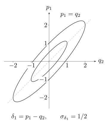
The two-mode example correlates $q_2$ with $p_1$. Contours satisfy $q_2^2+4(p_1-q_2)^2=1$ and $4$; the difference $\delta_1=p_1-q_2$ has standard deviation $1/2$. This is a two-variable marginal, not the full four-quadrature state.

Because the joint nullifier distribution is Gaussian with diagonal covariance, its two outcomes are independent. A joint window has probability

$$\Pr(|\delta_1|\leq1/2,|\delta_2|\leq1/2) =\operatorname{erf}(1/\sqrt2)^2\approx0.4660649427.$$

This tests the prepared resource state; it is not a logical algorithm’s success probability or an error-correction threshold.

Approximation, noise and computational cost

Finite squeezing uses finite energy. For momentum squeezing, $\operatorname{Var}(p)=e^{-2r}/2$, while $\operatorname{Var}(q)=e^{2r}/2$. The variance reduction relative to vacuum is $20r/\ln10$ decibels. Loss adds vacuum fluctuations and changes both resource-state correlations and any induced logical channel.

A finite cutoff cannot approximate oscillator operations uniformly on all states. One channel metric restricts the input mean occupation:

$$\|\Phi-\Psi\|_{\diamond E} =\sup_{\rho_{AR}:\,\operatorname{Tr}(\widehat N_A\rho_A)\leq E} \|[(\Phi-\Psi)\otimes\operatorname{id}_R](\rho_{AR})\|_1.$$

The reference system allows entangled inputs; $E$ is measured here in total photon-number units. This definition sets a comparison task, not an automatic convergence theorem. A concrete algorithm still needs a target, an input restriction, an error tolerance and a bound or convergence study. Unbounded-generator synthesis does not inherit a finite-dimensional Solovay–Kitaev estimate unchanged.

Costs include mode count, squeezing and energy, Gaussian operations, non-Gaussian preparation yield, measurement resolution, feedforward and postselection. Gaussian gate counts alone do not give laboratory runtime. Continuous-variable platforms treats sources, loss and detectors. GKP codes explains encoded qubit protection; an unencoded non-Gaussian gate is not already fault tolerant.

Exercises

Translate a Quadrature Convention

An author uses $[Q,P]=i/2$, vacuum covariance $I_2/4$, and reports

$$d_{QP} = \begin{pmatrix} 1\\ -1/2 \end{pmatrix}, \qquad V_{QP} = \operatorname{diag} \left( \frac14,1 \right).$$

Translate the state into this page’s convention, compute its mean photon number in both conventions, and identify one convention-invariant squeezing quantity.

Solution

The conventions are related by

$$q = \sqrt2\,Q, \qquad p = \sqrt2\,P.$$

First moments scale once and covariances twice:

$$d = \sqrt2\,d_{QP} = \begin{pmatrix} \sqrt2\\ -1/\sqrt2 \end{pmatrix}, \qquad V = 2V_{QP} = \operatorname{diag} \left( \frac12,2 \right).$$

The vacuum covariance correspondingly becomes $I_2/2$. In the first convention,

$$\bar n = \operatorname{Tr}V_{QP} + d_{QP}^{\mathsf T}d_{QP} - \frac12 = 2.$$

In the page convention,

$$\bar n = \frac{ \operatorname{Tr}V+d^{\mathsf T}d-1 }{2} = 2.$$

The ratio of a quadrature variance to the vacuum variance is invariant. Therefore a squeezing value in decibels is also invariant after the state and vacuum reference are translated together. A coefficient multiplying an unbounded gate generator would need its own dimensional translation and is not inferred here.

Compose an Affine Gaussian Circuit

Begin in vacuum. Apply a $q$-squeezer with $r=\ln2$, then rotate by $\pi/4$ using

$$R\left(\frac\pi4\right) = \frac1{\sqrt2} \begin{pmatrix} 1&-1\\ 1&1 \end{pmatrix},$$

and finally displace by $(1,-1/2)^{\mathsf T}$. Find the final mean, covariance, purity determinant, mean photon number, and probability that an ideal $q$-homodyne result lies in $[0,2]$.

Solution

The squeeze matrix is

$$S_{\rm sq} = \operatorname{diag} \left( \frac12,2 \right).$$

The total linear map is $R(\pi/4)S_{\rm sq}$ because the squeeze occurs first. The input mean is zero, and the final displacement occurs last, so

$$d = \begin{pmatrix} 1\\ -1/2 \end{pmatrix}.$$

Starting from $V_0=I_2/2$,

$$\begin{aligned} V &= R\left(\frac\pi4\right) S_{\rm sq}V_0S_{\rm sq}^{\mathsf T} R\left(\frac\pi4\right)^{\mathsf T} \\ &= \frac1{16} \begin{pmatrix} 17&-15\\ -15&17 \end{pmatrix}. \end{aligned}$$

Its determinant is $1/4$, as expected for a pure one-mode Gaussian state. The energy is

$$\bar n = \frac{ \operatorname{Tr}V+d^{\mathsf T}d-1 }{2} = \frac{19}{16}.$$

The $q$ outcome is normal with mean $1$ and variance $17/16$. The interval is symmetric about the mean, so

$$\begin{aligned} P(0\leq q\leq2) &= \operatorname{erf} \left( \frac{1}{\sqrt{2(17/16)}} \right) \\ &= \operatorname{erf} \left( \frac4{\sqrt{34}} \right) \\ &= 0.6680245329172630578\ldots. \end{aligned}$$

Reversing the matrix product would describe a different physical circuit.

Derive Three-Mode Line-Cluster Nullifiers

Prepare three independent momentum-squeezed vacua with $r=\ln2/2$. Apply unit-weight controlled phases on edges $(1,2)$ and $(2,3)$. Derive the three nullifiers, their covariance, the input and output mean photon numbers, and the preparation operations.

Solution

The two entanglers commute because they are functions of $q$ quadratures. Their Heisenberg action is

$$\begin{aligned} p_1' &= p_1+q_2, \\ p_2' &= p_2+q_1+q_3, \\ p_3' &= p_3+q_2, \end{aligned}$$

while every $q_j$ is unchanged. Hence

$$\begin{aligned} (\delta_1,\delta_2,\delta_3) &= (p_1'-q_2',\, p_2'-q_1'-q_3',\, p_3'-q_2') \\ &= (p_1,p_2,p_3). \end{aligned}$$

The input momenta are independent, so

$$\operatorname{Var}(\delta_j) = \frac14, \qquad \operatorname{Cov}(\delta_j,\delta_k) = 0 \quad (j\neq k).$$

Each input mode has mean photon number $1/8$, giving

$$\bar n_{\rm in} = \frac38.$$

For these inputs, each unit edge adds one mean photon. With two edges,

$$\bar n_{\rm cluster} = \frac38+2 = \frac{19}{8}.$$

The abstract preparation uses three modes, three squeezers, and two controlled-phase gates. It has no non-Gaussian resource and does not by itself implement a universal computation.

Propagate a Squeezed State through Pure Loss

A zero-mean one-mode state has $V_{\rm in}=\operatorname{diag}(1/8,2)$. Send it through a vacuum pure-loss channel with transmissivity $\eta=3/4$. Find the output covariance, determinant, mean photon number, and remaining $q$ squeezing.

Solution

For vacuum pure loss,

$$X = \sqrt{\eta}\,I_2, \qquad Y = \frac{1-\eta}{2}I_2.$$

Therefore

$$\begin{aligned} V_{\rm out} &= \frac34 \operatorname{diag} \left( \frac18,2 \right) + \frac18 I_2 \\ &= \operatorname{diag} \left( \frac7{32},\frac{13}{8} \right). \end{aligned}$$

The determinant is

$$\det V_{\rm out} = \frac{91}{256} > \frac14,$$

so the output is mixed. Its mean photon number is

$$\bar n_{\rm out} = \frac{ \operatorname{Tr}V_{\rm out}-1 }{2} = \frac{27}{64} = \frac34 \left( \frac9{16} \right).$$

The final $q$ variance $7/32$ remains below the vacuum value $1/2$, so some squeezing survives. The vacuum environment supplies the added noise; the mean occupation is reduced by the factor $\eta$.

Separate Gaussian Closure from Universality

Classify the following three model claims:

1. Gaussian input states, Gaussian gates and channels, homodyne with fixed settings, and affine displacement feedforward.
2. The same model with photon counting added.
3. Gaussian controls plus an available cubic interaction.

Explain whether each model remains within Gaussian closure, and what additional assumptions a universality claim needs.

Solution

The first model remains in Gaussian closure. With efficiently computable parameters and controlled arithmetic precision, its means, covariances and Gaussian outcome distributions admit efficient classical propagation. This does not make the states classical, but the declared operation set is not universal for arbitrary continuous-variable transformations.

Photon counting is a non-Gaussian measurement, so the second model leaves Gaussian closure. That fact alone does not give a universal gate set, efficient state preparation, useful postselection rate, fault tolerance, or an advantage result.

The third model meets the ideal algebraic premise used to generate polynomial Hamiltonians only after specifying available strengths, signs or inverses, common domains, energy-limited inputs, approximation accuracy, continuous-parameter precision, and commutator construction costs. Even then, algebraic universality does not supply an efficient compiler, physical implementation, or fault tolerance.

Bound a Fock-Space Truncation from Mean Energy

Use the cubic-phase example’s output energy $\bar n=3/8$. Bound the probability outside a cutoff retaining levels $0$ through $63$, and find the smallest cutoff parameter guaranteed by the same inequality to make the tail at most $10^{-3}$. Also bound the trace distance to the normalized projected state, and explain why this does not prove convergence of a truncated gate implementation.

Solution

Retaining levels $0,\ldots,63$ means $N=64$. Markov’s bound gives

$$\Pr(n\geq64) \leq \frac{3/8}{64} = \frac3{512} = 0.005859375.$$

For a guarantee of at most $10^{-3}$,

$$\frac{3}{8N} \leq 10^{-3},$$

so

$$N \geq 375.$$

For $N=64$, the trace distance is at most $\sqrt{3/512}\approx0.07655$. At $N=375$, the same bound is $\sqrt{10^{-3}}\approx0.03162$, not $10^{-3}$. A sufficient choice for trace-distance tolerance $10^{-3}$ is instead $N\geq375000$. These conservative guarantees compare the state with its normalized projection. Replacing the actual evolution by a truncated Hamiltonian is a separate approximation, requiring its own convergence check.

Count a Twenty-Five-Mode Cluster Wire

Prepare a path of twenty-five independent momentum-squeezed vacua with $r=\ln2/2$, join nearest neighbors by unit-weight controlled phases, measure the first twenty-four modes by homodyne, and retain one output. Count the model-level resources and compute the energy before and after entangling.

Solution

The path has twenty-five vertices and twenty-four edges. Its preparation uses twenty-five modes and squeezers and twenty-four controlled-phase gates. A path’s edges can be colored with two colors, so the entangling preparation has two gate layers if disjoint gates are parallel and shared-mode gates are not. The measurement stage consumes twenty-four modes, produces twenty-four real records, and leaves one quantum output. A fully sequential dependency declaration permits worst-case adaptive measurement depth twenty-four.

Each squeezed input has mean photon number $1/8$, hence

$$\bar n_{\rm in} = \frac{25}{8}.$$

Every unit path edge adds one mean photon for these input variances. Therefore

$$\bar n_{\rm cluster} = \frac{25}{8}+24 = \frac{217}{8}.$$

There is no non-Gaussian resource. Because no injected logical input, homodyne angles, or feedforward gains were given, these counts license only a Gaussian resource state and its measurement count, not a particular logical channel or fidelity. Physical loss, detector bandwidth, feedforward latency and actual hardware parallelism have not been specified by these ideal counts.

Decode a thresholded homodyne result

Start in vacuum, squeeze $q$ by $r=\ln2$, then displace it by $+1$. Measure $q$ and output bit one exactly when the result is nonnegative. Find the output probability, mean photon number before measurement and squeezing in decibels. Compare its error against target bit one with a Fock-tail bound at $N=16$.

Solution

The operations give $d=(1,0)^{\mathsf T}$ and $V=\operatorname{diag}(1/8,2)$. Hence $q\sim\mathcal N(1,1/8)$ and

$$\Pr(b=1)=\frac{1+\operatorname{erf}(2)}2 \approx0.9976611325.$$

The error is $0.0023388675$, also the total-variation distance to a point mass at one. The quantum state before measurement is Gaussian; thresholding its classical record produces a discrete Bernoulli output.

Its mean photon number is $[1/8+2+1-1]/2=17/16$. The squeezing is $20\ln2/\ln10\approx6.0206$ dB. Markov’s bound gives $\Pr(n\geq16)\leq17/256$, which concerns a different measurement and is not the decoded bit-error probability. A normalized projection at that cutoff has trace-distance bound $\sqrt{17/256}$; this loose guarantee also differs from the actual ideal program error.

References

• S. D. Bartlett, B. C. Sanders, S. L. Braunstein, and K. Nemoto, “Efficient Classical Simulation of Continuous Variable Quantum Information Processes,” Physical Review Letters 88, 097904 (2002), doi:10.1103/PhysRevLett.88.097904.
• M. Gu, C. Weedbrook, N. C. Menicucci, T. C. Ralph, and P. van Loock, “Quantum computing with continuous-variable clusters,” Physical Review A 79, 062318 (2009), doi:10.1103/PhysRevA.79.062318.
• S. Lloyd and S. L. Braunstein, “Quantum Computation over Continuous Variables,” Physical Review Letters 82, 1784–1787 (1999), doi:10.1103/PhysRevLett.82.1784.
• A. Mari and J. Eisert, “Positive Wigner Functions Render Classical Simulation of Quantum Computation Efficient,” Physical Review Letters 109, 230503 (2012), doi:10.1103/PhysRevLett.109.230503.
• N. C. Menicucci, P. van Loock, M. Gu, C. Weedbrook, T. C. Ralph, and M. A. Nielsen, “Universal Quantum Computation with Continuous-Variable Cluster States,” Physical Review Letters 97, 110501 (2006), doi:10.1103/PhysRevLett.97.110501.
• M. E. Shirokov, “Energy-constrained diamond norms and their use in quantum information theory,” arXiv:1706.00361 (2017), arXiv:1706.00361 — channel comparison with an input energy constraint.
• C. Weedbrook et al., “Gaussian quantum information,” Reviews of Modern Physics 84, 621–669 (2012), doi:10.1103/RevModPhys.84.621.