Continuous-Variable Platforms

A continuous-variable platform manipulates optical or microwave modes through their field quadratures. Squeezers, interferometers, coherent drives, and quadrature detectors provide a versatile set of Gaussian operations. The central hardware problem is to deliver the required state and measurement through loss, imperfect mode matching, phase drift, and finite control latency. An operation can run without heralded rejection even though its measurement outcomes remain random.

Gaussian processing alone does not give universal quantum computation. A suitable non-Gaussian resource and a way to consume it are also needed. A large entangled mode graph, a photon-counting sampler, and a protected logical qubit therefore require different performance tests. This page develops the optical and microwave mechanisms; Continuous-Variable Quantum Computation explains the computation models and approximation assumptions, while Bosonic Qubits treats finite-dimensional encodings in oscillators.

Helpful background. Bits, Qubits, Qudits, and Modes distinguishes information carriers; Continuous-Variable Systems introduces oscillator modes; Gaussian States and Wigner Functions develops the covariance description used below.

Modes and quadratures

For one mode with annihilation operator $a$, use

$$\begin{aligned} q &= \frac{a+a^\dagger}{\sqrt{2}}, \\ p &= \frac{a-a^\dagger}{i\sqrt{2}}. \end{aligned}$$

These obey

$$[q,p] = i, \qquad \operatorname{Var}_{0}(q) = \operatorname{Var}_{0}(p) = \frac{1}{2}.$$

Some literature uses vacuum variance $1$ or $1/4$. Raw covariances must be rescaled before combining such conventions. A decibel ratio $V_{\rm s}/V_{\rm vac}$ is unchanged by a common rescaling of both variances; comparing it still requires the same reference plane, bandwidth, and treatment of detector noise.

For $m$ modes, collect the quadratures into

$$\mathbf R = \left( q_1,p_1,\ldots,q_m,p_m \right)^{\mathsf T},$$

with commutators

$$[R_j,R_k] = i\Omega_{jk}, \qquad \Omega = \bigoplus_{j=1}^{m} \begin{pmatrix} 0&1\\ -1&0 \end{pmatrix}.$$

The first moments and covariance matrix are

$$\begin{aligned} d_j &= \langle R_j\rangle, \\ V_{jk} &= \frac{1}{2} \left\langle \{\Delta R_j,\Delta R_k\} \right\rangle. \end{aligned}$$

A mode is not merely a frequency label. It is a normalized field profile across time, frequency, space, and polarization. For temporal envelopes $u_j(t)$, orthogonality requires

$$\int dt\, u_j^*(t)u_k(t) = \delta_{jk}.$$

With $a_j=\int dt\,u_j^*(t)b(t)$ and $[b(t),b^\dagger(t')]=\delta(t-t')$,

$$[a_j,a_k^\dagger]=G_{jk},\qquad G_{jk}=\int dt\,u_j^*(t)u_k(t).$$

Thus overlapping bins are not independent canonical modes. Linearly independent profiles can be orthogonalized, but small eigenvalues of the overlap matrix make separation sensitive to noise. A comb’s number of spectral peaks does not by itself determine how many modes can be independently prepared, mixed, and read out.

Gaussian controls

A Gaussian unitary acts affinely on quadratures:

$$U^\dagger\mathbf R U = S\mathbf R+\mathbf s, \qquad S\Omega S^{\mathsf T} = \Omega.$$

The symplectic matrix $S$ describes phase rotations, squeezing, beam splitters, and multimode interferometers; $\mathbf s$ describes displacements. Means and covariances transform as

$$\begin{aligned} \mathbf d &\longmapsto S\mathbf d+\mathbf s, \\ V &\longmapsto SVS^{\mathsf T}. \end{aligned}$$

Means and covariances describe a Gaussian state completely. Gaussian preparation, quadratic Hamiltonians, and Gaussian measurements can be tracked efficiently, including suitable adaptive controls (Bartlett and colleagues). Conditional states remain Gaussian; arbitrary nonlinear classical processing of outcomes need not leave the outcome-averaged state Gaussian. Efficient simulation also assumes an efficiently computable controller and specified numerical precision.

Native operations and their hardware

Primitive	Ideal action	Representative hardware	Typical imperfections
displacement	$D(\alpha)$ translates phase space	weak coherent injection, directional coupler, electro-optic drive	gain error, phase drift, finite bandwidth
phase rotation	$a\mapsto e^{-i\phi}a$	phase shifter, propagation, detuning	phase noise, dispersion, calibration drift
single-mode squeezing	$q\mapsto e^{-r}q$, $p\mapsto e^r p$	optical parametric oscillator or phase-sensitive parametric amplifier	loss, pump noise, excess anti-squeezing
beam splitter	mixes two modes unitarily	directional coupler, free-space or fibre coupler, microwave hybrid	imbalance, mode mismatch, insertion loss
two-mode squeezing	correlated pair creation	parametric down-conversion, four-wave mixing, Josephson mixer	thermal population, spectral impurity, pump leakage
homodyne measurement	measures $q_\theta$	local oscillator and balanced detector, or phase-sensitive microwave readout	inefficiency, electronic noise, LO phase error
feedforward	conditional displacement or basis change	FPGA, ADC/DAC, modulator, microwave drive	latency, quantization, clipping, drift

Optical devices often provide low thermal occupation and room-temperature propagation. Microwave devices provide strong, tunable Josephson nonlinearities and direct compatibility with superconducting circuits, but they require cryogenic operation and quantum-limited amplification. These are different engineering trades, not merely different carrier frequencies.

Squeezing is a source metric, not a platform verdict

An ideal squeezed vacuum has

$$V_{\rm s} = \frac{1}{2}e^{-2r}, \qquad V_{\rm a} = \frac{1}{2}e^{2r}.$$

Noise suppression is often quoted as a positive number

$$\mathcal S_{\rm dB} = -10\log_{10} \left( \frac{V_{\rm s}}{V_{\rm vac}} \right).$$

A useful report includes both squeezing and anti-squeezing, because loss, phase jitter, pump noise, and impurity affect them differently. It also includes the analysis frequency, bandwidth, optical or microwave reference plane, detection correction, uncertainty, and duration of stable operation. An inferred source value corrected for detector loss is not the same as the variance delivered to the next module.

Non-Gaussian resources and computational tasks

Gaussian controls transform quadratures linearly. A cubic phase gate instead has the nonlinear Heisenberg action

$$\begin{aligned} U_3(\gamma)&=e^{i\gamma q^3},\\ U_3^\dagger qU_3&=q,\\ U_3^\dagger pU_3&=p+3\gamma q^2. \end{aligned}$$

Here $q,p,\gamma$ are dimensionless. The commutator $[p,q^3]=-3iq^2$ gives the last line; higher nested commutators vanish. A controllable suitable nonquadratic interaction together with a sufficiently rich Gaussian gate set supplies polynomial continuous-variable universality in the Lloyd–Braunstein construction. Its approximation and finite-energy assumptions matter: the label “non-Gaussian” alone is not a universal-gate-set proof.

In optics, preparing an ancilla and teleporting its action can replace a weak direct nonlinearity. Photon counting, photon-conditioned preparation, and finite-energy grid states are possible ingredients. Each has a different output state, success probability, and sensitivity to loss. Photon subtraction, for example, leaves a normalized coherent state unchanged because $a|\alpha\rangle=\alpha|\alpha\rangle$; it does not always generate non-Gaussianity. See Walschaers for resource preparation and GKP Codes for grid-state recovery.

Task	Physical resources	Quantity to test
Gaussian teleportation or sensing	squeezing, mode mixing, quadrature measurement, feedforward	channel noise or estimation error for specified input states
Cluster-state computation	finite-squeezed graph, adaptive measurement, suitable non-Gaussian resources for universality	implemented gate/channel error and accumulated noise
Gaussian boson sampling	squeezed inputs, interferometer, photon counting	output distribution and cost against specified classical algorithms
Encoded logical computation	finite-energy code states, recovery, and logical gates	logical error and accepted throughput as resources increase

Photon-number or threshold detection can make the readout of a Gaussian state non-Gaussian. This can support sampling tasks without implementing arbitrary logical gates. Conversely, an oscillator carrying one encoded qubit is not counted as an unlimited register merely because its Hilbert space is infinite-dimensional. Dated grid-state and recovery developments are discussed in Bosonic Codes in Research.

Optical implementations

Sources and interferometers

Optical squeezing is commonly produced below threshold in an optical parametric oscillator or in a travelling-wave nonlinear medium. Second-order down-conversion and third-order four-wave mixing create correlated photon pairs, which become single- or two-mode squeezed states in an appropriate mode basis. Integrated microrings and waveguides can place source, interferometer, filtering, and phase control on a chip; bulk or fibre systems can offer lower loss or easier access during development.

The source must be characterized in the mode accepted by the processor. Spectral entanglement between an intended pulse and unobserved modes appears as mixedness. Filtering can improve purity while reducing brightness and adding loss. Pump depletion, thermal drift, parasitic nonlinear processes, and Raman or fluorescence backgrounds can make a nominally Gaussian source depart from its calibration model.

A passive $m$-mode interferometer implements

$$\mathbf a_{\rm out} = U\mathbf a_{\rm in}, \qquad U^\dagger U = I_m.$$

The matrix $U$ may be realized spatially by a mesh of beam splitters and phase shifters, temporally by recirculating delay loops, or spectrally by electro-optic modulation and pulse shaping. The abstract unitary does not show insertion loss, switching loss, finite extinction, phase-lock channels, or the number of times a pulse traverses a lossy component. Those belong in the physical transfer matrix.

Time-domain multiplexing

Time-domain multiplexing reuses one or a few squeezers, beam splitters, and detectors across a pulse train. If the clock period is $\tau$, a delay of $k\tau$ couples bins separated by $k$ steps. Several delays generate a graph with long-range edges while keeping the number of physical components nearly fixed.

This economy transfers complexity into:

• optical delay length and propagation loss;
• fast switching and phase modulation;
• clock and local-oscillator synchronization;
• accumulation of phase error over many traversals;
• detector recovery and demultiplexing;
• real-time feedforward before the target pulse leaves its delay.

Temporal depth is not automatically circuit depth. A cluster resource may contain a long stream of entangled modes while the demonstrated measurement pattern acts on only a subset or uses fixed bases.

Frequency-domain multiplexing

An optical frequency comb supplies many spectral modes from one resonator. Pump frequencies determine which mode pairs interact, and shaped polychromatic local oscillators select supermodes at readout. This can create dense or reconfigurable graphs without long spatial interferometers.

A shaped local oscillator measures a selected superposition of spectral modes. Changing that superposition does not automatically supply independent control of every coupling. Covariance measurements, mode-selectivity measurements, dispersion, and pump-induced cross-talk determine which of the nominal modes can be used together.

Cluster states and adaptive processing

For a real symmetric adjacency matrix $A$, with zero diagonal for a graph without self-loops, define

$$\delta_j=p_j-\sum_k A_{jk}q_k.$$

The commutator is $[\delta_j,\delta_k]=i(A_{kj}-A_{jk})=0$. This is why the graph must have the specified symmetry: its ideal nullifiers can be simultaneously sharp. The formal state obeying $\delta_j|\psi_A\rangle=0$ for every $j$ has infinite squeezing and is not a normalizable finite-energy preparation.

A useful finite-energy construction starts with independently momentum-squeezed modes and applies controlled-phase couplings. They send $p\mapsto p+Aq$ and leave $q$ unchanged, so the output nullifiers inherit the input momentum noise. In the ideal construction with equal squeezing $r$,

$$\operatorname{Var}(\delta_j)=\frac12e^{-2r}.$$

Real optical networks can realize differently weighted or rescaled nullifiers; the measured coefficients and shot-noise normalization must accompany the variance. Entanglement requires violation of an applicable separability inequality, not merely a small-looking variance or a large graph. Van Loock–Furusawa gives variance criteria; the exact partitions excluded by a witness must be specified. Gaussian-state reconstruction from first and second moments additionally assumes Gaussianity.

Finite squeezing becomes noise in gate teleportation. More nodes do not remove that noise. Encoding and recovery must handle it together with loss, envelope distortion, and non-Gaussian faults. The constructions of Menicucci and colleagues and Gu and colleagues explain the graph-to-gate mapping; Asavanant and Larsen and their collaborators give optical implementations of two-dimensional resource graphs.

Feedforward sets a delay requirement

A later quadrature angle or displacement can depend on an earlier measurement. Let $\tau_{\rm ff}$ be the time from that measurement to a settled conditional actuator, including conversion, computation, and a timing margin. If the target pulse already arrives after a delay $\tau_{\rm existing}$, extra fibre of group index $n_g$ must supply

$$L_{\rm extra}\geq\frac{c}{n_g} \max(0,\tau_{\rm ff}-\tau_{\rm existing}).$$

Longer delay increases propagation loss and phase sensitivity. Component propagation already included in $\tau_{\rm existing}$ reduces the extra fibre requirement; it is not an additional electronic latency. A long entangled pulse train therefore need not imply a long sequence of successfully adapted logical gates.

Microwave implementations

Microwave continuous-variable systems use propagating or resonant modes in superconducting circuits. Josephson parametric amplifiers, Josephson parametric converters, and Josephson travelling-wave parametric amplifiers provide strong three- or four-wave mixing. Hybrid rings, circulators, directional couplers, transmission lines, and digital IQ chains implement mode mixing and measurement.

Thermal occupation

At frequency $\omega$ and temperature $T$, equilibrium thermal occupation is

$$\bar n_{\rm th} = \frac{1} {\exp\!\left(\hbar\omega/k_{\rm B}T\right)-1}.$$

Optical modes have negligible $\bar n_{\rm th}$ at room temperature. Microwave modes near a few gigahertz require millikelvin environments, cold attenuation, filtering, and careful isolation from warmer amplifier stages. The refrigerator base temperature alone does not determine the mode temperature; cable loss, pump leakage, imperfect thermalization, and backaction can raise it.

Parametric sources and frequency graphs

A pumped Josephson element can implement the two-mode-squeezing interaction

$$H_{\rm TMS} = i\hbar \left( g a_j^\dagger a_k^\dagger -g^*a_ja_k \right).$$

Multiple pump tones select multiple frequency pairs and therefore program an interaction graph. This provides a compact route to microwave frequency combs and cluster-like states, but pump crowding introduces intermodulation, gain competition, harmonics, and calibration complexity.

Two-mode microwave sources and separated output lines are described by Eichler and Flurin and their collaborators. For the displayed Hamiltonian, $g$ is a complex coupling rate and the rotating-wave/pump approximation must be valid.

Amplification and quadrature readout

A quantum-limited phase-preserving amplifier has a dilation

$$a_{\rm out}=\sqrt G\,a_{\rm in} +\sqrt{G-1}\,b_{\rm in}^\dagger, \qquad G\geq1.$$

The second term is required to preserve $[a_{\rm out},a_{\rm out}^\dagger]=1$. With an independent vacuum idler, either quadrature’s output variance divided by $G$ is

$$\frac{V_{\rm out}}G=V_{\rm in}+\frac{1-G^{-1}}2.$$

Thus the input-referred added noise approaches half a quantum at high gain (Caves). Thermal idler occupation or an inefficient chain increases it. A phase-sensitive amplifier can amplify one quadrature without this same added-noise requirement by deamplifying its conjugate.

An ordinary simultaneous IQ record is a two-quadrature measurement, not an ideal homodyne sample of a freely chosen single quadrature. For ideal heterodyne detection, expressed as quadrature estimates in the present normalization,

$$V_{\rm estimates}=V+\frac12 I.$$

Here $V_{\rm estimates}$ is the classical covariance matrix of the two-component outcome vector. The extra vacuum contribution follows from splitting the signal with vacuum and rescaling both readout arms. Electronics and amplifier noise must be referred to the same input before comparing detectors. Subtracting a calibrated noise contribution can estimate source moments; it does not physically restore a transmitted state or remove uncertainty and drift.

Preparing and measuring resources

Initialization

Gaussian initialization can be deterministic: cool or evacuate the mode, displace it, squeeze it, and entangle it with other modes. Non-Gaussian initialization is usually more costly. Photon detection may herald a conditioned optical state; a superconducting ancilla may synthesize a cavity state; breeding or distillation may combine several imperfect resources.

For a heralded resource with per-attempt probability $p_{\rm h}$, multiplexing $N$ independent attempts gives

$$p_{\geq 1} = 1-(1-p_{\rm h})^N.$$

This improves availability only if successful states can be routed into the processor with sufficiently low loss and latency. Switches, buffers, and discarded attempts are part of the cost.

Gates

Gaussian gates can be direct interferometric transformations or measurement-induced operations. A non-Gaussian gate can be teleported from an ancilla, conditioned on a detector result, or mediated by a nonlinear matter degree of freedom. The reported gate error should include ancilla quality, coupling loss, detector error, feedforward, and any acceptance rule.

An operation demonstrated on coherent or squeezed probes need not have the same fidelity on a Wigner-negative input. Process characterization should cover the energy and phase-space region used by the algorithm or logical code.

Homodyne, heterodyne, and photon counting

Homodyne detection measures one quadrature selected by a local-oscillator phase. It can be efficient and fast, but phase error rotates anti-squeezed noise into the measured quadrature. Heterodyne detection obtains both quadratures at the cost of an additional vacuum contribution in the ideal model.

Photon-number resolving detection supplies a non-Gaussian measurement. Its relevant metrics are system efficiency, number resolution, dark counts, timing jitter, saturation, reset time, and maximum sustainable event rate. A detector with excellent intrinsic efficiency can still sit behind lossy coupling, filtering, switching, and interferometry.

Loss, phase jitter, and finite resources

Loss is mixing with an environment

A thermal attenuator has $a_{\rm out}=\sqrt\eta\,a_{\rm in}+\sqrt{1-\eta}\,b$, with independent thermal environment $b$. Its power transmissivity is $0\leq\eta\leq1$. The moments obey

$$\begin{aligned} d_{\rm out}&=\sqrt\eta\,d_{\rm in},\\ V_{\rm out}&=\eta V_{\rm in} +(1-\eta)\left(\bar n_{\rm env}+\frac12\right)I. \end{aligned}$$

Only complete loss $\eta=0$ replaces an arbitrary input by the environment state. With vacuum loss, a coherent input remains the pure coherent state $|\sqrt\eta\alpha\rangle$; other inputs can become mixed. Non-Gaussian features may weaken or disappear, depending on state and attenuation. The channel is not a universal state-independent “success with probability $\eta$” followed by a harmless flagged failure.

For serial scalar attenuators acting on the same selected mode, power transmissivities multiply: $\eta_{\rm tot}=\prod_j\eta_j$. Added thermal noise must also be propagated through later stages. Mode mixing and correlated environments require a multimode description, as developed in Gaussian Channels.

More squeezing can increase phase sensitivity

For a zero-mean state with covariance diagonal in its squeezed axes, a fixed angular error gives

$$V(\delta\theta)=V_{\rm s}\cos^2\delta\theta +V_{\rm a}\sin^2\delta\theta.$$

For zero-mean Gaussian phase jitter of standard deviation $\sigma_\theta$ radians, independent of the state, define $c_\theta=e^{-2\sigma_\theta^2}$. Averaging the rotation gives

$$\overline V= \frac{V_{\rm s}+V_{\rm a}}2 +\frac{V_{\rm s}-V_{\rm a}}2c_\theta.$$

This uses $\langle\cos2\delta\theta\rangle=c_\theta$. Nonzero fluctuating displacements add a further variance of the conditional mean. For an ideal squeezed vacuum, the normalized noise is

$$2\overline V= \frac{1+c_\theta}{2}e^{-2r} +\frac{1-c_\theta}{2}e^{2r}.$$

The first term decreases with $r$, while the second grows. At $\sigma_\theta>0$ the optimum is

$$r_* =\frac14\log\frac{1+c_\theta}{1-c_\theta}, \qquad 2\overline V_{\min}=\sqrt{1-c_\theta^2}.$$

Subsequent vacuum loss changes this normalized variance to $1-\eta+2\eta\overline V$. For fixed $\eta>0$, it leaves the optimizing $r_*$ unchanged. At $\sigma_\theta=2^\circ$ and $\eta=0.90$, about $14.6$ dB of ideal source squeezing gives the best observed value, about $7.88$ dB. Increasing the source to $20$ dB makes the observed value worse.

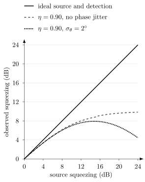
Loss alone limits the observed noise suppression to $10$ dB for $\eta=0.90$. Independent Gaussian phase jitter with standard deviation $2^\circ$ also mixes in anti-squeezed noise, producing an optimum at finite source squeezing. The input is an ideal pure squeezed vacuum; excess source noise would change these curves.

Mode mismatch and electronic limits

A detector matched to the wrong wave packet measures a superposition of the desired mode and orthogonal modes. This is equivalent to simple vacuum loss only when those other modes are uncorrelated vacuum. Occupied or correlated unwanted modes can instead introduce excess noise and cross-talk. Mode selectivity should therefore be measured under the pump, switching, and local-oscillator conditions used in the experiment.

Finite squeezing adds noise to cluster teleportation and broadens approximate grid-state peaks. It is not removed by increasing the number of modes. Pump fluctuations, clipping, finite converter resolution, and finite bandwidth can further make noise correlated or nonstationary. Control, Readout, and Calibration discusses how to measure these effects.

Heralded resources have a conditional rate

For one well-defined attempt per clock cycle, let a resource be ready with probability $p_{\rm ready}$, let a required detection occur with conditional probability $p_{\rm registered\mid ready}$, and let the recorded event pass the selection rule with probability $p_{\rm accepted\mid registered,ready}$. Then

$$\begin{aligned} R_{\rm acc}&=R_{\rm clock}\,p_{\rm joint},\\ p_{\rm joint}&=p_{\rm ready} p_{\rm registered\mid ready} {}\times p_{\rm accepted\mid registered,ready}. \end{aligned}$$

These conditional factors are a probability identity, without an independence assumption. Optical power transmission may enter a single-photon detection probability, but it cannot generally be substituted for a CV state’s survival probability. For example, an ideal detector clicks on an attenuated coherent pulse with probability $1-e^{-\eta|\alpha|^2}$, not $\eta$. Several simultaneous resource requirements, waiting, and buffering need their actual joint statistics.

Characterizing a useful multimode device

Generating a correlated graph, programming its couplings, and measuring selected modes adaptively are distinct capabilities. A source can produce many correlated spectral modes while the available controls address only a few global supermodes. A time loop can provide distant graph edges while accumulated loss limits usable depth.

Covariance data provide a strong consistency check:

$$V+\frac{i}{2}\Omega\succeq0.$$

This condition is necessary for every quantum state with finite second moments and sufficient for a covariance to define a Gaussian state. Violations beyond measurement uncertainty indicate a reconstruction or calibration problem. Passing it does not establish Gaussianity. The purity formula

$$\operatorname{Tr}\rho^2=\frac{1}{\sqrt{\det(2V)}}$$

applies to Gaussian states; a pure one-photon Fock state has $V=3I/2$, for which the right-hand side is $1/3$, not its actual purity $1$.

A useful comparison therefore pairs the squeezed and anti-squeezed variances with the selected mode functions, energy, bandwidth, loss, and uncertainty. For a Gaussian cluster, test the intended correlations with an appropriate separability bound. For a non-Gaussian ancilla, characterize the finite-energy target and the operation that consumes the state. A sampling experiment requires distribution tests and an explicit classical comparison; an encoded processor requires logical error versus resources, including rejected attempts. Metrics for Quantum Hardware develops the statistical interpretation.

Optical propagation, microwave nonlinearities, and multiplexing each offer useful capabilities. Their value depends on the actual task: low inferred source noise does not guarantee low delivered noise, and high pulse rate does not guarantee high accepted logical throughput.

Exercises

1. Verify the quadrature convention

Starting from $[a,a^\dagger]=1$, verify $[q,p]=i$ for the quadratures used on this page. Show that the vacuum variances are $1/2$.

Solution

The commutator is

$$\begin{aligned} [q,p] &= \frac{1}{i2} [a+a^\dagger,a-a^\dagger] \\ &= \frac{1}{i2} \left( -[a,a^\dagger] +[a^\dagger,a] \right) \\ &= i. \end{aligned}$$

Since $a\lvert0\rangle=0$ and $\langle0\rvert aa^\dagger\lvert0\rangle=1$,

$$\langle q^2\rangle_0 = \langle p^2\rangle_0 = \frac{1}{2},$$

while both means vanish.

2. Send squeezed light through loss

An optical source produces $10\ {\rm dB}$ of ideal squeezing and then passes through a vacuum-loss channel with $\eta=0.80$. What squeezing is observed?

Solution

Ten decibels means

$$\frac{V_{\rm s}}{V_{\rm vac}} = 10^{-10/10} = 0.1.$$

Vacuum loss gives

$$\frac{V_{{\rm s,out}}}{V_{\rm vac}} = \eta(0.1)+(1-\eta) = 0.28.$$

Therefore

$$\mathcal S_{\rm out} = -10\log_{10}(0.28) \approx 5.53\ {\rm dB}.$$

A $20\%$ loss removes almost half of the quoted noise suppression in decibel terms.

3. Quantify phase-jitter contamination

A state has $V_{\rm s}=0.05$ and $V_{\rm a}=5.0$ in units where vacuum variance is $0.5$. Find the observed variance for a fixed phase error of $2^\circ$. Compare it with the ideal squeezed variance.

Solution

Using $\delta\theta=2\pi/180$,

$$\begin{aligned} V(\delta\theta) &= 0.05\cos^2\delta\theta + 5.0\sin^2\delta\theta \\ &\approx 0.0560. \end{aligned}$$

The variance increases by about $12\%$. The absolute angle is small, but the large anti-squeezed variance amplifies its effect.

4. Compare microwave thermal occupations

Estimate $\bar n_{\rm th}$ for a $5\ {\rm GHz}$ mode at $20\ {\rm mK}$ and $100\ {\rm mK}$. Use $h f/k_{\rm B}\approx0.240\ {\rm K}$.

Solution

At fixed frequency,

$$\bar n_{\rm th} = \frac{1}{e^{hf/(k_{\rm B}T)}-1}.$$

At $20\ {\rm mK}$,

$$\bar n_{\rm th} \approx \frac{1}{e^{12}-1} \approx 6.1\times10^{-6}.$$

At $100\ {\rm mK}$,

$$\bar n_{\rm th} \approx \frac{1}{e^{2.4}-1} \approx 0.10.$$

The fivefold temperature increase changes the mode from nearly vacuum to roughly one thermal photon per ten modes on average.

5. Check a beam splitter

For

$$\begin{pmatrix} a_1'\\ a_2' \end{pmatrix} = \begin{pmatrix} \sqrt{\eta}&\sqrt{1-\eta}\\ -\sqrt{1-\eta}&\sqrt{\eta} \end{pmatrix} \begin{pmatrix} a_1\\ a_2 \end{pmatrix},$$

verify that $[a_j',a_k'^\dagger]=\delta_{jk}$.

Solution

The mixing matrix $U$ is real and satisfies

$$UU^\dagger = \begin{pmatrix} \eta+1-\eta&0\\ 0&1-\eta+\eta \end{pmatrix} = I.$$

Therefore

$$\begin{aligned} [a_j',a_k'^\dagger] &= \sum_{\ell,m} U_{j\ell}U_{km}^* [a_\ell,a_m^\dagger] \\ &= (UU^\dagger)_{jk} \\ &= \delta_{jk}. \end{aligned}$$

The minus sign makes the rows orthogonal in this real-amplitude convention. Other beam-splitter conventions place the relative phase in complex reflection amplitudes.

6. Size an optical feedforward delay

A controller has latency $64$ ns including its timing margin. The target pulse already reaches the conditional actuator $24$ ns after the relevant measurement. Find the extra fibre length for group index $n_g=1.5$. Compare with a setup having no existing delay.

Solution

The added delay is $64-24=40$ ns, so

$$\begin{aligned} L_{\rm extra}&=\frac{c}{n_g}(40\ {\rm ns})\\ &=8.0\ {\rm m}. \end{aligned}$$

With no existing delay, the requirement is $12.8$ m. Extra electronic latency or a larger margin increases the required length; propagation delay already present in the target arm reduces it. The measurement and target clocks must use the same timing origin.

7. Compound an efficiency budget

A heralded single photon passes through coupling with efficiency $0.95$, three loop traversals each with efficiency $0.97$, a switch with efficiency $0.94$, and a detector with efficiency $0.98$. Find the end-to-end efficiency.

Solution

The efficiencies multiply:

$$\begin{aligned} \eta_{\rm tot} &= 0.95 (0.97)^3 (0.94) (0.98) \\ &\approx 0.798. \end{aligned}$$

Thus about $20\%$ of these single-photon detection events are lost even though every component has at least $94\%$ efficiency. The same product is a power transmissivity for a general optical mode, not a universal state-fidelity formula.

8. Interpret a cluster nullifier

For a three-node line with unit-weight edges, write the three nullifiers. What does a measured nonzero variance mean?

Solution

With edges $1$–$2$ and $2$–$3$,

$$\begin{aligned} \delta_1 &= p_1-q_2, \\ \delta_2 &= p_2-q_1-q_3, \\ \delta_3 &= p_3-q_2. \end{aligned}$$

An ideal infinitely squeezed cluster state would have zero variance for every nullifier. A physical nonzero variance reflects finite squeezing plus loss, phase error, mode mismatch, and detector noise. The independent vacuum reference gives variances $1$, $3/2$, and $1$ for these three unnormalized nullifiers. Reduced noise shows correlations relative to that reference. Entanglement requires an applicable separability inequality, and universal computation requires additional operations.

9. Compute accepted resource throughput

A source is clocked at $10\ {\rm MHz}$. It heralds a single-photon ancilla with probability $0.02$. That photon must traverse a path of transmissivity $0.75$ and be detected with efficiency $0.95$; $80\%$ of the registered events then pass a selection rule. Neglect dark counts and other branches. Estimate the accepted rate.

Solution

The schematic rate is

$$\begin{aligned} p_{\rm tot} &= (0.02)(0.75)(0.95)(0.80) \\ &= 0.0114, \\ R_{\rm acc} &= (10^7\ {\rm s^{-1}})p_{\rm tot} \\ &= 1.14\times10^5\ {\rm s^{-1}}. \end{aligned}$$

The useful rate is $114\ {\rm kHz}$, not the $10\ {\rm MHz}$ source clock. If several independent ancillas are needed simultaneously, the rate can fall much more sharply unless multiplexing is included.

10. Find the optimum squeezing with phase jitter

For ideal input squeezing, derive $r_*$ above by minimizing the phase-averaged variance. What happens as $\sigma_\theta\to0$? Does attenuation of fixed transmissivity change $r_*$?

Solution

Write $2\overline V=Ae^{-2r}+Be^{2r}$ with $A=(1+c_\theta)/2$ and $B=(1-c_\theta)/2$. Setting its derivative to zero gives $e^{4r_*}=A/B$. The second derivative is positive. At the minimum,

$$2\overline V_{\min}=2\sqrt{AB}=\sqrt{1-c_\theta^2}.$$

For small nonzero $\sigma_\theta$, $B\simeq\sigma_\theta^2$, $r_*\simeq-\tfrac12\log\sigma_\theta$, and the normalized minimum is approximately $2\sigma_\theta$. As jitter vanishes, the optimum moves to infinite squeezing; no finite optimum remains in the ideal source model. Fixed vacuum loss multiplies the objective by $\eta$ and adds $1-\eta$, so it leaves the optimum unchanged for $\eta>0$. At complete loss every input gives vacuum.

11. Check what covariance can establish

Compare the one-photon state and a thermal state of mean occupation $1$. Can their covariances or energies distinguish them? Can their purities?

Solution

Both have zero mean, $V=3I/2$, and $\langle n\rangle=1$. The Fock state is pure and non-Gaussian. The thermal state has probabilities $p_n=2^{-(n+1)}$ and purity

$$\sum_{n=0}^{\infty}p_n^2 =\frac{1/4}{1-1/4}=\frac13.$$

Its Gaussian covariance formula gives that same result. Distinguishing the states needs information beyond second moments, such as photon-number statistics: their $\langle n(n-1)\rangle$ values are $0$ and $2$.

References

• W. Asavanant et al., “Generation of Time-Domain-Multiplexed Two-Dimensional Cluster State,” Science 366, 373–376 (2019), doi:10.1126/science.aay2645.

• S. D. Bartlett, B. C. Sanders, S. L. Braunstein, and K. Nemoto, “Efficient Classical Simulation of Continuous Variable Quantum Information Processes,” Physical Review Letters 88, 097904 (2002), doi:10.1103/PhysRevLett.88.097904.

• S. L. Braunstein and P. van Loock, “Quantum Information with Continuous Variables,” Reviews of Modern Physics 77, 513–577 (2005), doi:10.1103/RevModPhys.77.513.

• C. M. Caves, “Quantum Limits on Noise in Linear Amplifiers,” Physical Review D 26, 1817–1839 (1982), doi:10.1103/PhysRevD.26.1817.

• C. Eichler et al., “Observation of Two-Mode Squeezing in the Microwave Frequency Domain,” Physical Review Letters 107, 113601 (2011), doi:10.1103/PhysRevLett.107.113601.

• E. Flurin, N. Roch, F. Mallet, M. H. Devoret, and B. Huard, “Generating Entangled Microwave Radiation over Two Transmission Lines,” Physical Review Letters 109, 183901 (2012), doi:10.1103/PhysRevLett.109.183901.

• A. Furusawa et al., “Unconditional Quantum Teleportation,” Science 282, 706–709 (1998), doi:10.1126/science.282.5389.706.

• D. Gottesman, A. Kitaev, and J. Preskill, “Encoding a Qubit in an Oscillator,” Physical Review A 64, 012310 (2001), doi:10.1103/PhysRevA.64.012310.

• M. Gu, C. Weedbrook, N. C. Menicucci, T. C. Ralph, and P. van Loock, “Quantum Computing with Continuous-Variable Clusters,” Physical Review A 79, 062318 (2009), doi:10.1103/PhysRevA.79.062318.

• M. V. Larsen, X. Guo, C. R. Breum, J. S. Neergaard-Nielsen, and U. L. Andersen, “Deterministic Generation of a Two-Dimensional Cluster State,” Science 366, 369–372 (2019), doi:10.1126/science.aay4354.

• S. Lloyd and S. L. Braunstein, “Quantum Computation over Continuous Variables,” Physical Review Letters 82, 1784–1787 (1999), doi:10.1103/PhysRevLett.82.1784.

• L. S. Madsen et al., “Quantum Computational Advantage with a Programmable Photonic Processor,” Nature 606, 75–81 (2022), doi:10.1038/s41586-022-04725-x.

• N. C. Menicucci, “Fault-Tolerant Measurement-Based Quantum Computing with Continuous-Variable Cluster States,” Physical Review Letters 112, 120504 (2014), doi:10.1103/PhysRevLett.112.120504.

• N. C. Menicucci et al., “Universal Quantum Computation with Continuous-Variable Cluster States,” Physical Review Letters 97, 110501 (2006), doi:10.1103/PhysRevLett.97.110501.

• H. Vahlbruch et al., “Detection of 15 dB Squeezed States of Light and Their Application for the Absolute Calibration of Photoelectric Quantum Efficiency,” Physical Review Letters 117, 110801 (2016), doi:10.1103/PhysRevLett.117.110801.

• P. van Loock and A. Furusawa, “Detecting Genuine Multipartite Continuous-Variable Entanglement,” Physical Review A 67, 052315 (2003), doi:10.1103/PhysRevA.67.052315.

• M. Walschaers, “Non-Gaussian Quantum States and Where to Find Them,” PRX Quantum 2, 030204 (2021), doi:10.1103/PRXQuantum.2.030204.

• C. Weedbrook et al., “Gaussian Quantum Information,” Reviews of Modern Physics 84, 621–669 (2012), doi:10.1103/RevModPhys.84.621.