Superconducting Qubits

Superconducting qubits encode information in selected levels of electrical circuits. A Josephson element supplies nonlinearity; capacitance, inductance, couplers, and electromagnetic ports determine the spectrum, controls, and losses. The main design tradeoff is between sensitivity to noise and the ability to prepare, distinguish, and couple the chosen states. This page compares circuit families and explains how multilevel physics affects a processor, without ranking current performance records.

Required background. Hardware Overview explains physical encodings and operations; Josephson Effect supplies junction and flux conventions; Circuit QED Overview develops circuit quantization and resonator coupling.

Charge, phase, and circuit levels

For one effective superconducting mode, a useful starting form is

$$H=4E_C(n-n_g)^2+U(\phi).$$

For an isolated superconducting island, $n$ counts excess Cooper pairs, $n_g$ is an offset charge in units of $2e$, and $E_C=e^2/(2C_\Sigma)$. The phase is compact: $e^{i\phi}|n\rangle=|n+1\rangle$ and $[n,e^{i\phi}]=e^{i\phi}$ are globally well-defined rotor relations. Writing $[\phi,n]=i$ is a local phase-coordinate shorthand, not a global canonical commutator for an angle and an integer spectrum.

For a mode shunted by an ideal linear inductance, the flux coordinate can instead range over the real line, with $n=-i\partial_\phi$ and $[\phi,n]=i$ on a suitable common domain. In either model the Josephson energy contributes $-E_J\cos\phi$, but the coordinate domain and boundary conditions affect the spectrum.

In a multimode circuit, $n$ and $\phi$ become vectors and the capacitance and inductance networks determine coupled normal modes. The Josephson cosine mixes those modes and makes their level spacings unequal. The qubit is a selected pair of eigenstates of this full circuit, not a literal microscopic two-state object.

Three design choices recur:

1. Choose an operating coordinate. Charge-like, flux-like, and phase-like circuits couple differently to control fields and noise.
2. Engineer a quiet point. A transition frequency may be first-order insensitive to offset charge or applied flux at a chosen bias.
3. Retain enough anharmonicity. The $0\leftrightarrow1$ transition must be controllable without unacceptable excitation of nearby levels.

Increasing insensitivity in one coordinate usually changes matrix elements, frequencies, control speed, footprint, or sensitivity to another mechanism. There is no context-free best ratio of circuit energies.

Transmons, flux qubits, and fluxonium

Transmons

A transmon is a Josephson junction, often a split junction, shunted by a comparatively large capacitance. Its Hamiltonian is

$$H_{\mathrm{tr}} = 4E_C(n-n_g)^2 - E_J\cos\phi.$$

In the regime $E_J/E_C\gg1$, the low-energy spectrum is approximately

$$\begin{aligned} \hbar\omega_{01} &\approx \sqrt{8E_JE_C}-E_C, \\ \alpha &\equiv \omega_{12}-\omega_{01} \approx -\frac{E_C}{\hbar}. \end{aligned}$$

Large $E_J/E_C$ suppresses charge dispersion exponentially, which made the transmon much less sensitive to offset-charge noise than the Cooper-pair box. The relative anharmonicity $|\alpha|/\omega_{01}$ becomes small. Increasing $E_J$ alone at fixed $E_C$ does not reduce the leading absolute $|\alpha|=E_C/\hbar$, whereas increasing the shunt capacitance reduces $E_C$. Fast or spectrally broad pulses can populate $|2\rangle$ and higher states. Koch and colleagues derive these distinct scalings.

Fixed-frequency transmons avoid a dedicated flux-bias degree of freedom and can reduce flux-noise sensitivity, but fabrication spread must be accommodated by frequency allocation and microwave-activated interactions. Flux-tunable transmons replace one junction by a SQUID so that an effective $E_J(\Phi)$ and therefore the transition frequency can be changed. Tunability helps activate gates and avoid some collisions, but moving away from a flux sweet spot increases dephasing and exposes the system to waveform distortion and parasitic crossings.

Circuit QED Overview derives the spectrum, charge dispersion, multilevel dispersive shift, and controlled two-level truncation. This page uses the transmon as one component of a larger architecture.

Persistent-current flux qubits

A conventional flux qubit uses a superconducting loop interrupted by several Josephson junctions. Near half a flux quantum, localized states with opposite circulating currents form a useful two-state basis. They are not generally the energy eigenstates: tunneling mixes them. In this persistent-current basis, a reduced model is

$$H_{\mathrm{fq}} = -\frac{1}{2} \left( \Delta\sigma_x + \epsilon\sigma_z \right),$$

with

$$\epsilon \approx 2I_p \left( \Phi_{\mathrm{ext}}-\frac{\Phi_0}{2} \right).$$

$I_p$ is the persistent-current magnitude, $\Delta>0$ is a tunneling energy (not an angular frequency), and $\Phi_0=h/(2e)$ is the superconducting flux quantum. At the degeneracy point $\epsilon=0$, the transition frequency is first-order insensitive to flux. Away from it, the magnetic moment provides strong tunability and coupling but also converts low-frequency flux fluctuations into dephasing.

Capacitively shunted flux qubits and related designs interpolate between traditional flux circuits and transmon-like devices. “Flux qubit” therefore does not identify one Hamiltonian, noise sensitivity, or gate stack; the circuit and operating point must be stated.

Fluxonium

Fluxonium adds a large linear inductive shunt, often realized by a Josephson-junction array or another superinductance, to a smaller junction. A one-mode model is

$$H_{\mathrm{fl}} = 4E_Cn^2 + \frac{E_L}{2} (\phi-\phi_{\mathrm{ext}})^2 - E_J\cos\phi.$$

In this ideal noncompact one-mode model, a static offset $n_g$ can be removed by a unitary phase factor $e^{in_g\phi}$ without changing boundary conditions. This explains static offset-charge insensitivity; it does not remove time-dependent electric noise or effects of array phase slips and extra modes. Manucharyan and colleagues state the conditions under which the junction array behaves as an inductive shunt. The cosine and parabolic potential can produce strong anharmonicity. Depending on the energy ratios and flux bias, fluxonium can offer long-lived transitions, large separation from leakage levels, and useful selection rules. It can also operate at comparatively low transition frequency, require a large or complex inductive element, and present gate, readout, fabrication, and frequency-allocation constraints different from transmons.

Here $\phi_{\mathrm{ext}}=2\pi\Phi_{\mathrm{ext}}/\Phi_0$ is the dimensionless external-flux coordinate in the displayed convention. Other circuit-quantization conventions may distribute signs and flux offsets differently, so compare physical spectra rather than symbols alone.

Fluxonium is an active processor platform, not a single settled design. Heavy-fluxonium, integer-fluxonium, and coupler architectures make different choices about transition frequency, flux bias, matrix elements, protection, and interaction strength. Component coherence or a two-qubit demonstration does not by itself establish large-array yield and control.

Family comparison

Family	Primary design idea	Useful feature	Architectural pressure
fixed-frequency transmon	large capacitive shunt and fixed $E_J$	charge-noise suppression; microwave-only one-qubit control	fabrication spread, frequency crowding, always-on interactions
tunable transmon	SQUID-controlled effective $E_J$	frequency steering and flux-activated gates	flux noise, pulse distortion, parasitic level crossings
persistent-current flux qubit	opposite circulating-current states	strong magnetic coupling and flux control	flux-noise sensitivity and bias distribution
fluxonium	Josephson element plus superinductance	strong anharmonicity and noise-insensitive operating points	inductor complexity, distinct gate/readout stack, extra array modes and circuit-dependent control
protected or encoded circuit	symmetry, interference, or enlarged circuit suppresses selected errors	biased or reduced sensitivity to a chosen channel	preparation, control, readout, extra modes, fabrication complexity

The final row includes several research programs rather than one device. Protection is always conditional: identify the suppressed operator, the remaining channels, and the controls that may break the protection.

Initialization and Reset

At thermal equilibrium, an ideal two-level transition has

$$\frac{p_1}{p_0} = \exp\!\left( -\frac{\hbar\omega_{01}}{k_{\mathrm B}T} \right).$$

Microwave-frequency qubits are therefore operated in dilution refrigerators. The base-plate temperature, however, is not automatically the qubit temperature. Incomplete attenuation, infrared radiation, quasiparticles, resonator photons, poor thermalization, and measurement bias can produce excess excited-state population.

Cryogenic and Vacuum Infrastructure explains how cooling stages, attenuation, and shielding determine the electromagnetic environment.

Initialization options include:

• passive waiting for energy relaxation;
• measurement followed by conditional correction;
• resonator-assisted or sideband reset;
• engineered dissipation;
• transfer through an auxiliary level or lossy mode.

Reset is a channel with duration, residual excitation, leakage, induced photons, and spectator effects. Fast ancilla reuse in repeated error correction makes the complete reset-plus-readout latency more relevant than passive $T_1$ alone. Control, Readout, and Calibration explains reset channels and evolution during feedback delay.

Microwave control of a selected transition

A microwave voltage or current couples through a charge-like or flux-like circuit operator. For the computational basis use $Z=|0\rangle\langle0|-|1\rangle\langle1|$, so the free qubit Hamiltonian is $-\hbar\omega_{01}Z/2$. Set $\delta=\omega_{\mathrm{drive}}-\omega_{01}$. In the drive frame and under the rotating-wave approximation,

$$\frac{H_{\mathrm{rot}}(t)}{\hbar} = \frac{\delta(t)}{2}Z + \frac{\Omega_x(t)}{2}X + \frac{\Omega_y(t)}{2}Y.$$

The in-phase and quadrature envelopes set the rotation angle and equatorial axis. A software frame update implements many logical $Z$ rotations without a physical waiting period. Physical accuracy still depends on oscillator phase, channel delay, mixer calibration, transfer functions, detuning, drive-induced shifts, and spectator response.

Weak transmon anharmonicity makes pulse shaping important. Smooth envelopes reduce spectral spillover; derivative quadratures can suppress leading leakage and phase errors; virtual frame corrections remove deterministic phases. A successful isolated Rabi fit is only the beginning. Long sequences and simultaneous operation must test coherent accumulation, leakage, and crosstalk.

Fluxonium and flux qubits can have different transition matrix elements and selection rules. A pulse family that works for a transmon cannot be transferred by matching only the qubit frequency.

Entangling interactions and leakage levels

Superconducting circuits can couple capacitively, inductively, through a resonator or bus, or through a dedicated nonlinear coupler. After eliminating inactive modes and choosing a frame, a schematic effective interaction is

$$\frac{H_{\mathrm{eff}}}{\hbar} = \frac{J_x}{2}X_1X_2 + \frac{J_y}{2}Y_1Y_2 + \frac{\zeta}{4}Z_1Z_2 + \frac{H_{\mathrm{drive}}}{\hbar} +\cdots.$$

Here $J_x,J_y,\zeta$ have angular-frequency units. Driven interactions can add other terms, such as $ZX$ in cross-resonance operation. The gate protocol activates and times selected terms while suppressing residual coupling, unwanted conditional phases, spectator interactions, and transitions involving $\lvert2\rangle$ or coupler levels.

Strategy	Typical mechanism	Strength	Main risks
cross-resonance	drive one fixed-frequency qubit near a neighbor’s transition	avoids flux tuning of data qubits	unwanted Hamiltonian terms, spectator effects, frequency constraints
flux-pulsed controlled phase	tune levels near an avoided crossing	direct and fast conditional phase	leakage, flux noise, pulse distortion, collision history
parametric exchange or phase gate	modulate a qubit or coupler near a difference or sum frequency	frequency-selective activation	sidebands, ac shifts, modulation crosstalk
tunable coupler	vary an intermediate mode or effective interaction	high on/off ratio and flexible gate families	coupler leakage, added calibration, residual $ZZ$, extra control line
resonator-mediated gate	use virtual or driven bus photons	can connect separated circuit nodes	photon loss, residual population, crowding, correlated phases

Gate labels such as CNOT, CZ, iSWAP, and echoed cross-resonance name ideal logical operations. A hardware report must also state duration, echoed or compiled construction, frame updates, leakage treatment, simultaneous context, and characterization protocol.

Tunable coupling solves one problem by adding another controllable quantum mode. Its frequency, anharmonicity, transfer function, thermal state, and leakage paths become part of the calibration graph. Likewise, fixed-frequency control removes flux excursions but places more burden on fabrication yield, microwave selectivity, and cancellation of static interactions.

A controlled phase through an avoided crossing

The noncomputational level $|02\rangle$ can be useful rather than merely an error. Suppose two weakly anharmonic modes have exchange interaction $\hbar J(b_1^\dagger b_2+b_1b_2^\dagger)$, with real $J>0$. Near an isolated $|11\rangle$–$|02\rangle$ crossing, subtract the bare $|11\rangle$ energy and write

$$\frac{H_{\mathrm{pair}}}{\hbar} =\begin{pmatrix}0&\sqrt2J\\\sqrt2J&\delta_{02}\end{pmatrix}, \qquad \delta_{02}=\omega_2+\alpha_2-\omega_1.$$

The factor $\sqrt2$ comes from $b_2^\dagger|1\rangle=\sqrt2|2\rangle$. This reduction requires other states, especially $|20\rangle$, to be sufficiently far detuned. Its eigenvalues are

$$\frac{E_\pm}{\hbar} =\frac{\delta_{02}\pm\sqrt{\delta_{02}^2+8J^2}}2.$$

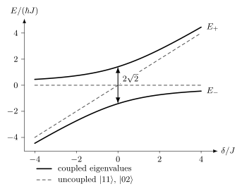
The horizontal and diagonal dashed lines are the uncoupled $|11\rangle$ and $|02\rangle$ energies. Coupling opens a minimum gap $2\sqrt2\hbar J$. The plotted detuning $\delta$ denotes $\delta_{02}$. Following a dressed branch shifts the phase of the computational component; a rapid pulse can instead produce a coherent excursion into $|02\rangle$ and back.

For constant resonant coupling, $\delta_{02}=0$, an initial $|11\rangle$ evolves as

$$|\psi(t)\rangle=\cos(\sqrt2Jt)|11\rangle -i\sin(\sqrt2Jt)|02\rangle.$$

At $t=\pi/(\sqrt2J)$ it returns with phase $-1$ and zero final leakage, despite reaching full $|02\rangle$ population halfway through. A controlled-Z results only if the other computational amplitudes return appropriately and their single-qubit phases are corrected. Real pulse ramps, other crossings, decay of $|02\rangle$, and spectator coupling must be included. The zero-leakage endpoint alone does not establish a high-fidelity gate. Blais and colleagues review these multilevel gate mechanisms.

Dispersive resonator readout

For an ideal two-level qubit coupled to a resonator, let $\Delta_r=\omega_q-\omega_r$ and $\chi=g^2/\Delta_r$, with all three quantities in angular-frequency units. Under $|\Delta_r|\gg g\sqrt{n+1}$, the Hamiltonian through second order is, up to a scalar,

$$\frac{H_{\mathrm{disp}}}{\hbar} \simeq(\omega_r-\chi Z)a^\dagger a -\frac{\omega_q+\chi}{2}Z.$$

This uses the same ground-positive $Z$ as the control equation. Texts using an excited-positive Pauli operator write the opposite signs. The resonator frequencies conditioned on ground and excited qubit states are $\omega_r-\chi$ and $\omega_r+\chi$, respectively. A probe therefore produces distinguishable output fields, which are amplified, digitized, and classified.

For a transmon the nearby $|2\rangle$ state changes both the conditional separation and the common resonator shift. The two-level value $g^2/\Delta_r$ is generally insufficient. Circuit QED Overview derives the multilevel result and explains why the transmon conditional shift cannot simply replace every occurrence of the two-level Lamb shift.

Increasing probe power improves distinguishability only within the validity of the model: large photon number can cause transitions or invalidate dispersive mixing. The resonator’s photon-number decay rate $\kappa$ sets its Lorentzian angular-frequency linewidth; its field amplitude decays at $\kappa/2$. For $|\Delta_r|\gg g,\kappa$ and a simple Markovian output port, the qubit-like excitation has photon admixture approximately $(g/\Delta_r)^2$, giving

$$\Gamma_{\mathrm P}\simeq\kappa(g/\Delta_r)^2.$$

A Purcell filter changes the impedance at the qubit frequency while retaining a readout path. Multiplexing also couples resonator spacing, amplifier dynamic range, ring-down time, and crosstalk. Quantum Instruments explains why accurate assignment does not guarantee preservation of the measured state.

Relaxation, dephasing, and leakage

Energy relaxation

For weak Markovian loss channels coupled to independent baths, downward rates add approximately. At negligible thermal excitation,

$$\frac{1}{T_1} = \sum_j\Gamma_j.$$

A participation-ratio model for dielectric loss gives the schematic contribution

$$\Gamma_{\mathrm{diel}} \approx \omega_{01} \sum_i p_i\tan\delta_i,$$

where $p_i$ is the fraction of electric-field energy in region or material $i$, and $\tan\delta_i$ is its effective loss tangent under the measurement conditions. This model motivates reducing electric-field participation in lossy interfaces, but fitted participation does not uniquely identify a microscopic defect.

Other relaxation channels include:

• Purcell and other radiative loss through control or readout ports;
• nonequilibrium quasiparticle tunneling;
• resonant two-level defects and package modes;
• conductor, seam, and vortex loss;
• phonon and substrate coupling;
• drive-induced heating and leakage-assisted decay.

At nonzero thermal excitation, population relaxation toward equilibrium has $T_1^{-1}=\Gamma_\downarrow+\Gamma_\uparrow$, rather than the downward rate alone. Strongly coupled defects and structured modes can invalidate a single exponential. $T_1$ may also vary with frequency, time, cooldown, package, radiation environment, and nearby device activity. A maximum value selected from a sweep is not a stationary processor error rate.

Dephasing and sweet spots

If the transition frequency depends on fluctuating parameters $\lambda_j$, then to first order

$$\delta\omega_{01} \approx \sum_j \frac{\partial\omega_{01}}{\partial\lambda_j} \delta\lambda_j.$$

At a sweet spot, one derivative vanishes. Second-order sensitivity, noise in other coordinates, photon shot noise, control-reference noise, and discrete fluctuators remain. Low-frequency flux or charge noise often produces nonexponential Ramsey decay, so one fitted $T_2^\ast$ should not be promoted to a universal dephasing rate.

Under a simple Markovian decomposition,

$$\frac{1}{T_2} = \frac{1}{2T_1} + \frac{1}{T_\phi}.$$

Use this identity only when the protocol and noise model support it. Ramsey, echo, dynamical-decoupling, and driven-gate experiments sample different spectral bands.

Leakage and correlated faults

Leakage is population outside the declared computational subspace. In transmons it commonly involves $\lvert2\rangle$ and higher states; in coupled circuits it can also occupy a bus or coupler. Leakage can persist across cycles, spread phase errors to neighbors, and violate a decoder’s assumed two-level noise model. Report leakage and seepage separately from in-subspace infidelity.

Correlations can arise from shared control electronics, common readout lines, residual $ZZ$, package modes, heating, quasiparticle diffusion, and energetic radiation events. A fault that affects many qubits at once may be rare in wall-clock time yet disproportionately important for a large code. Device-level noise therefore needs spatial and temporal correlation tests, not only marginal $T_1$ and randomized-benchmarking averages.

Connectivity and frequency allocation

Planar superconducting circuits naturally provide a sparse geometric graph. Qubits couple to selected neighbors through direct capacitances or inductances, resonators, or dedicated couplers. Typical degree is limited because every added connection consumes area, creates additional modes and collision conditions, and changes crosstalk and calibration.

Usable couplings, residual interactions, disabled components, and simultaneous-operation exclusions determine which schedule can run. A design graph alone omits those physical constraints.

Frequency allocation is a graph problem

Transition frequencies cannot be assigned independently. A usable allocation should avoid or control:

• equal or nearly equal neighboring transitions when selectivity requires separation;
• collisions between a qubit’s $0\leftrightarrow1$ transition and a neighbor’s $1\leftrightarrow2$ transition;
• resonances involving couplers, buses, readout modes, sidebands, and multiphoton processes;
• crowded readout resonators on a shared feedline;
• trajectories through unwanted avoided crossings during flux pulses;
• frequencies with strong loss from a defect or package mode.

Fabrication variation turns this into a yield problem. Frequency tunability can recover some devices, but it also changes coherence, residual coupling, readout detuning, and the location of every pulse-dependent collision. Laser trimming, post-fabrication tuning, replaceable modules, and calibration-aware compilation address different parts of the problem.

Parallelism is measured, not inferred

Disjoint graph edges are not automatically executable in parallel. Simultaneous microwave tones can cause Stark shifts, amplifier compression, classical leakage, or spurious transitions. Flux pulses can share return paths or distort neighboring biases. Readout can populate common modes and dephase spectators.

Parallel schedules should be characterized directly. A useful report compares isolated and simultaneous gates, includes spectator states, and records which combinations the compiler forbids. “Nearest-neighbor connectivity” does not specify this concurrency graph.

Packaging and cryogenic constraints

The qubit mode extends into pads, ground planes, wirebonds, bumps, enclosures, and nearby dielectrics. Packaging is therefore part of the Hamiltonian and loss budget. It must:

• suppress slotline, box, substrate, and interposer modes;
• provide dense ground connections and controlled impedances;
• thermalize conductors while limiting heat flow to the cold stage;
• attenuate incoming thermal noise and infrared radiation;
• route outgoing signals through isolation and low-noise amplification;
• avoid magnetic vortices, dissipative seams, and lossy surface participation;
• remain manufacturable and testable at acceptable yield.

Edge wiring becomes difficult for a large two-dimensional array because interior sites need drive, flux, coupler, and readout access. Air bridges, multilayer wiring, flip-chip bonding, superconducting bumps, through-silicon vias, interposers, and chiplets move signals into the third dimension. Each added layer can also introduce dielectric loss, unwanted modes, thermal resistance, bond variability, and new failure sites.

The refrigerator has finite cooling power at each stage. Every cable contributes conducted heat; attenuators dissipate control power; amplifiers and circulators occupy cold volume; readout bandwidth and output power are finite. Cryogenic classical electronics may reduce cable count and latency, but its power, noise, fabrication, and thermal interfaces must be included.

Modularity reduces some die-size and fabrication pressures, while introducing a communication channel with its own loss, noise, latency, and calibration. Interconnects and Transduction compares physical links, and Modular Architectures explains how their errors and timing affect distributed operations.

Repeated error correction on a local graph

The Surface Code uses local parity checks on a two-dimensional graph, repeated measurement, reset, and classical decoding. Those requirements align with several strengths of superconducting circuits:

• patterned local couplings;
• fast programmable gates relative to many atomic platforms;
• integrated resonator readout;
• mid-circuit measurement and active reset;
• electronic feedforward and frame tracking;
• planar fabrication compatible with repeated unit cells.

The alignment is not automatic. A useful syndrome cycle also requires:

• a gate order that limits hook errors and crosstalk;
• measurement qubits that reset without contaminating data qubits;
• leakage removal or leakage-aware decoding;
• stable operation over many repeated rounds;
• a decoder whose throughput keeps up and whose latency meets conditional-operation deadlines;
• correlated-noise characterization;
• logical scaling measured across code distances.

For the usual rotated planar patch of odd distance $d$, the ideal layout has $d^2$ data and $d^2-1$ measurement qubits, totaling

$$N_{\mathrm{phys}} = 2d^2-1$$

data and measurement qubits for one logical memory, before routing, boundaries between logical patches, magic-state factories, spares, and other architecture overheads. The formula is a layout count, not a resource estimate for an algorithm.

What improving a logical memory establishes

Lower measured logical error at larger code distance tests a particular memory circuit, noise regime, and decoder. Compare matched operating conditions and uncertainty, including leakage, postselection, and repeated-round behavior. The result does not by itself establish universal logical gates, state injection, reliable interconnects, or the resources for an algorithm. Surface-Code Thresholds explains these conditions; Quantum Hardware Scaling maintains dated experimental assessments.

Other codes trade connectivity, measurement weight, decoder complexity, noise bias, and qubit overhead differently. A local superconducting graph is useful for surface-code checks, but does not select a code independently of those constraints.

Worked spectrum, temperature, and relaxation estimate

Consider a transmon design with

$$\frac{E_C}{h} = 250\,\mathrm{MHz}, \qquad \frac{E_J}{E_C} = 50.$$

Then $E_J/h=12.5\,\mathrm{GHz}$, and the leading transmon estimate gives

$$\begin{aligned} \frac{\omega_{01}}{2\pi} &\approx \frac{\sqrt{8E_JE_C}-E_C}{h} \\ &= 5.00\,\mathrm{GHz} - 0.25\,\mathrm{GHz} \\ &= 4.75\,\mathrm{GHz}, \end{aligned}$$

with

$$\frac{\alpha}{2\pi} \approx -250\,\mathrm{MHz}.$$

This is a design estimate. Spectroscopy must identify the actual transitions, nearby modes, and device-to-device spread.

At equilibrium temperature $T=20\,\mathrm{mK}$, the ideal two-level population ratio is

$$\frac{p_1}{p_0} = \exp\!\left( -\frac{h(4.75\,\mathrm{GHz})} {k_{\mathrm B}(20\,\mathrm{mK})} \right) \approx 1.1\times10^{-5}.$$

At an effective temperature of $60\,\mathrm{mK}$, the same ratio is about $2.2\times10^{-2}$. This large difference is why base temperature cannot substitute for qubit thermometry. Even an effective-temperature fit is only a model when quasiparticle or drive-induced populations are present.

Now suppose $T_1=150\,\mu\mathrm{s}$ and a repeated syndrome cycle lasts $t_c=1.1\,\mu\mathrm{s}$. A qubit held in $\lvert1\rangle$ for the full cycle would relax with probability

$$\begin{aligned} p_{\mathrm{relax}} &= 1-e^{-t_c/T_1} \\ &\approx 7.3\times10^{-3}. \end{aligned}$$

For an arbitrary driven schedule with a constant Markovian downward rate $1/T_1$, the mean number of relaxation jumps is instead

$$\mu_\downarrow =\frac1{T_1}\int_0^{t_c}\rho_{11}(t)\,dt =\frac{\bar q\,t_c}{T_1},$$

where $\bar q$ is the time-averaged excited population of the actual ensemble state. The probability of at least one downward jump obeys $P(N_\downarrow\ge1)\le\mu_\downarrow$ and is approximately equal when multiple jumps are negligible. With $\bar q=0.4$, this gives $\mu_\downarrow\approx2.93\times10^{-3}$.

The expression $q(1-e^{-t_c/T_1})$ is exact for an undriven initial mixture with excitation probability $q$ and no upward transitions; there $q$ is the initial population, not its time average. Neither a jump probability nor its mean count is a logical error probability. Gates, measurement, recovery, dephasing, and correlations determine the computational consequence.

Exercises

1. Estimate a transmon spectrum

A transmon has $E_C/h=220\,\mathrm{MHz}$ and $E_J/E_C=60$. Estimate $\omega_{01}/2\pi$ and $\alpha/2\pi$ using the leading large-$E_J/E_C$ formulas.

Solution

First,

$$\frac{E_J}{h} = 60(0.220\,\mathrm{GHz}) = 13.2\,\mathrm{GHz}.$$

Therefore

$$\begin{aligned} \frac{\omega_{01}}{2\pi} &\approx \sqrt{8(13.2)(0.220)}\,\mathrm{GHz} - 0.220\,\mathrm{GHz}\\ &\approx 4.60\,\mathrm{GHz}. \end{aligned}$$

The anharmonicity estimate is

$$\frac{\alpha}{2\pi} \approx -\frac{E_C}{h} = -220\,\mathrm{MHz}.$$

These are asymptotic design values. A circuit model and spectroscopy are needed for precision and for identifying other modes.

2. Compare equilibrium populations

For a $5.0\,\mathrm{GHz}$ two-level transition, estimate the equilibrium excited-state population at $20\,\mathrm{mK}$ and $60\,\mathrm{mK}$.

Solution

For a two-level system,

$$p_1 = \frac{1} {1+e^{hf/(k_{\mathrm B}T)}}.$$

Since $hf/k_{\mathrm B}\approx0.240\,\mathrm K$, at $20\,\mathrm{mK}$,

$$p_1 \approx \frac{1}{1+e^{12.0}} \approx 6.1\times10^{-6}.$$

At $60\,\mathrm{mK}$,

$$p_1 \approx \frac{1}{1+e^{4.00}} \approx 1.8\times10^{-2}.$$

The threefold temperature increase changes the equilibrium population by roughly three orders of magnitude. A measured population need not be thermal, so this comparison is a diagnostic model rather than proof of a temperature.

3. Verify a flux sweet spot

For the effective flux-qubit splitting

$$E(\delta\Phi) = \sqrt{ \Delta^2 + (2I_p\delta\Phi)^2 },$$

show that $\delta\Phi=0$ is first-order insensitive to flux and find the leading small-$\delta\Phi$ correction.

Solution

Differentiation gives

$$\frac{dE}{d(\delta\Phi)} = \frac{4I_p^2\delta\Phi} {\sqrt{\Delta^2+(2I_p\delta\Phi)^2}},$$

which vanishes at $\delta\Phi=0$. Expanding the square root,

$$\begin{aligned} E(\delta\Phi) &= \Delta \sqrt{ 1+ \frac{4I_p^2\delta\Phi^2}{\Delta^2} } \\ &\approx \Delta + \frac{2I_p^2}{\Delta} \delta\Phi^2. \end{aligned}$$

The linear sensitivity is removed, but quadratic flux sensitivity and other noise channels remain.

4. Accumulate residual conditional phase

Two idle qubits have residual interaction

$$\frac{H_{ZZ}}{\hbar} = \frac{\zeta}{4}Z_1Z_2, \qquad \frac{\zeta}{2\pi} = 50\,\mathrm{kHz}.$$

What conditional phase magnitude accumulates during $2.0\,\mu\mathrm{s}$?

Solution

For this convention, the two-qubit conditional phase magnitude is $\lvert\zeta t\rvert$. Thus

$$\begin{aligned} \lvert\phi_{ZZ}\rvert &= 2\pi (50\times10^3) (2.0\times10^{-6}) \\ &= 0.2\pi \approx 0.628\,\mathrm{rad}. \end{aligned}$$

The signed nonlocal phase is $\phi_{00}-\phi_{01}-\phi_{10}+\phi_{11}=-\zeta t$. Independent single-qubit $Z$ frame changes leave this combination unchanged, so they cannot cancel it. An ideal midpoint $X$ echo on one qubit reverses $ZZ$ during the second half; a compensating two-qubit interaction, coupler adjustment, or different schedule can also reduce it. Finite echo pulses and spectator interactions require further analysis.

5. Estimate a simple Purcell limit

In the ideal two-level dispersive estimate,

$$\Gamma_{\mathrm P} \approx \kappa \left( \frac{g}{\Delta} \right)^2.$$

Take $g/2\pi=100\,\mathrm{MHz}$, $\lvert\Delta\rvert/2\pi=1.0\,\mathrm{GHz}$, and $\kappa/2\pi=5.0\,\mathrm{MHz}$. Estimate the Purcell-limited $T_1$.

Solution

The mixing ratio is $g/\lvert\Delta\rvert=0.1$, so

$$\frac{\Gamma_{\mathrm P}}{2\pi} \approx (5.0\,\mathrm{MHz})(0.1)^2 = 50\,\mathrm{kHz}.$$

Consequently,

$$T_{1,\mathrm P} = \frac{1}{\Gamma_{\mathrm P}} \approx \frac{1}{2\pi(50\,\mathrm{kHz})} \approx 3.2\,\mu\mathrm{s}.$$

This deliberately simple result shows the readout-speed tradeoff. Multilevel corrections and the actual frequency-dependent impedance, including a Purcell filter, are required for device design.

6. Bound jumps using the actual occupation

A qubit has constant downward rate $1/T_1$ with $T_1=200\,\mu\mathrm{s}$. A driven cycle lasts $1.0\,\mu\mathrm{s}$ and its actual time-averaged excited population is $\bar q=0.5$. Find the mean number of downward jumps and a bound on the probability of one or more.

Solution

$$\mu_\downarrow=\bar q\,t_c/T_1 =2.5\times10^{-3},\qquad P(N_\downarrow\ge1)\le2.5\times10^{-3}.$$

The bound follows from $N_\downarrow\ge\mathbf1_{N_\downarrow\ge1}$. Multiple jumps require re-excitation, which the drive may supply. Their probability determines how closely the bound is approached. A decoder’s logical error is a separate quantity.

7. Color a square coupling graph

Show why two alternating qubit-frequency bands can separate every nearest-neighbor pair on an ideal square lattice. Then name two reasons that this does not solve frequency allocation for a transmon processor.

Solution

The square lattice is bipartite: color each vertex by the parity of its integer coordinates. Every nearest-neighbor edge joins opposite parity, so assigning frequency band $A$ to one color and $B$ to the other makes neighboring $0\leftrightarrow1$ bands different.

This does not control collisions involving $1\leftrightarrow2$ transitions, couplers, readout resonators, sidebands, or multiphoton processes. It also leaves same-band next-nearest neighbors that can interact through crosstalk or shared modes. Fabrication spread broadens both bands, and simultaneous-gate protocols may require more than pairwise separation.

8. Return from a leakage level with a phase

For the isolated resonant pair $|11\rangle,|02\rangle$, take $J/(2\pi)=20\,\mathrm{MHz}$. Find the first return time with phase $-1$, the time of maximum $|02\rangle$ population, and the effect of doubling the return time.

Solution

The return time is $t_\pi=\pi/(\sqrt2J)=1/(2\sqrt2\times20\,\mathrm{MHz})\approx17.7\,\mathrm{ns}$. At $t_\pi/2\approx8.84\,\mathrm{ns}$, all population is in $|02\rangle$. At $2t_\pi$ the state returns with phase $+1$, so this ideal excursion no longer contributes a controlled-$\pi$ phase. These times omit ramps and assume the other states are decoupled; finite decay during the excursion cannot be repaired merely by returning its population.

References

• A. Blais, A. L. Grimsmo, S. M. Girvin, and A. Wallraff, “Circuit quantum electrodynamics,” Reviews of Modern Physics 93, 025005 (2021), doi:10.1103/RevModPhys.93.025005.
• G. Catelani, R. J. Schoelkopf, M. H. Devoret, and L. I. Glazman, “Relaxation and frequency shifts induced by quasiparticles in superconducting qubits,” Physical Review B 84, 064517 (2011), doi:10.1103/PhysRevB.84.064517.
• J. M. Chow et al., “Simple all-microwave entangling gate for fixed-frequency superconducting qubits,” Physical Review Letters 107, 080502 (2011), doi:10.1103/PhysRevLett.107.080502.
• A. Gyenis et al., “Moving beyond the transmon: Noise-protected superconducting quantum circuits,” PRX Quantum 2, 030101 (2021), doi:10.1103/PRXQuantum.2.030101.
• M. Kjaergaard et al., “Superconducting qubits: Current state of play,” Annual Review of Condensed Matter Physics 11, 369–395 (2020), doi:10.1146/annurev-conmatphys-031119-050605.
• J. Koch et al., “Charge-insensitive qubit design derived from the Cooper pair box,” Physical Review A 76, 042319 (2007), doi:10.1103/PhysRevA.76.042319.
• P. Krantz et al., “A quantum engineer’s guide to superconducting qubits,” Applied Physics Reviews 6, 021318 (2019), doi:10.1063/1.5089550.
• V. E. Manucharyan, J. Koch, L. I. Glazman, and M. H. Devoret, “Fluxonium: Single Cooper-pair circuit free of charge offsets,” Science 326, 113–116 (2009), doi:10.1126/science.1175552.
• J. M. Martinis et al., “Decoherence in Josephson qubits from dielectric loss,” Physical Review Letters 95, 210503 (2005), doi:10.1103/PhysRevLett.95.210503.
• D. C. McKay et al., “Universal gate for fixed-frequency qubits via a tunable bus,” Physical Review Applied 6, 064007 (2016), doi:10.1103/PhysRevApplied.6.064007.
• J. E. Mooij, T. P. Orlando, L. Levitov, L. Tian, C. H. van der Wal, and S. Lloyd, “Josephson persistent-current qubit,” Science 285, 1036–1039 (1999), doi:10.1126/science.285.5430.1036.
• D. Rosenberg et al., “3D integrated superconducting qubits,” npj Quantum Information 3, 42 (2017), doi:10.1038/s41534-017-0044-0.
• T. Walter et al., “Rapid high-fidelity single-shot dispersive readout of superconducting qubits,” Physical Review Applied 7, 054020 (2017), doi:10.1103/PhysRevApplied.7.054020.
• F. Yan et al., “Tunable coupling scheme for implementing high-fidelity two-qubit gates,” Physical Review Applied 10, 054062 (2018), doi:10.1103/PhysRevApplied.10.054062.