Josephson Effect

The Josephson effect turns a phase difference into a supercurrent and a voltage into phase evolution. A superconducting weak link can therefore carry a stationary current at zero voltage, oscillate under voltage bias and interfere with another coherent path. Its behavior depends on both the microscopic junction and the surrounding circuit.

We develop conventional equilibrium junctions first, then explain where harmonics, switching and driven occupations change that picture. A weak link may be an insulating barrier, a normal metal, a semiconductor, a ferromagnet or a constriction; these do not share one universal current–phase relation.

Required background. London Theory supplies gauge-invariant superflow and flux; BCS Theory supplies the paired reservoirs and excitation gap. Helpful background. Gauge Transformations explains phase and potential transformations.

Gauge-invariant phase across a weak link

Let $e>0$, so electrons have charge $-e$ and the flux quantum is $\Phi_0=h/(2e)$. Write the pair fields as $\Delta_j=|\Delta_j|e^{i\theta_j}$. For a path from electrode 1 to electrode 2, choose

$$\phi=\theta_1-\theta_2 -\frac{2e}{\hbar}\int_1^2\mathbf A\cdot d\boldsymbol\ell.$$

Under $\mathbf A\mapsto\mathbf A+\nabla\chi$ and $\theta_j\mapsto\theta_j-2e\chi_j/\hbar$, the changes cancel. Positive conventional current flows from 1 to 2. Take the voltage in the passive circuit orientation, so positive $IV$ is power entering the junction:

$$\dot\phi=\frac{2e}{\hbar}V.$$

Here $V$ is the electrochemical junction voltage; with matched equilibrium reservoirs and negligible additional chemical-potential imbalance, it reduces to the oriented electromagnetic voltage. Reversing the junction orientation reverses $\phi$, $I$ and $V$ together.

A useful two-mode picture has a pair-transfer term

$$\begin{aligned} H_{\rm link}&=-K\mathcal W_{12}\Psi_1^*\Psi_2+\mathrm{c.c.},\\ \mathcal W_{12}&=\exp\left[\frac{2ie}{\hbar} \int_1^2\mathbf A\cdot d\boldsymbol\ell\right]. \end{aligned}$$

For real $K>0$ and nearly fixed $\Psi_j=\sqrt{N_j}e^{i\theta_j}$, this is $-2K\sqrt{N_1N_2}\cos\phi$. Number–phase dynamics then gives a sinusoidal transfer current. This argument explains the phase dependence, but material transparency, geometry and gap structure determine its coefficient.

Current, energy and inductance

For a conventional tunnel junction,

$$\begin{aligned} I_s&=I_c\sin\phi,\\ U_J&=-E_J\cos\phi,\\ E_J&=\frac{\hbar I_c}{2e}. \end{aligned}$$

A static phase supports $|I_s|\leq I_c$ at zero voltage. More generally, equilibrium current follows the junction free energy:

$$I_s=\frac{2e}{\hbar}\frac{\partial F_J}{\partial\phi}.$$

This sign also ensures $dU_J/dt=I_sV$. The differential inductance about a static phase $\phi_0$ is

$$L_J(\phi_0)=\frac{\Phi_0}{2\pi I_c\cos\phi_0}.$$

It relates current to the circuit branch flux $\varphi_J=(\Phi_0/2\pi)\phi$, whose derivative is voltage. This branch coordinate is not the magnetic flux through the physical barrier. Negative differential inductance can be stabilized by another circuit element; stability depends on the total energy under the actual bias constraint.

For identical isotropic BCS electrodes and a low-transparency insulating barrier, the Ambegaokar–Baratoff result is

$$I_c(T)R_N=\frac{\pi\Delta(T)}{2e} \tanh\frac{\Delta(T)}{2k_BT}.$$

$R_N$ is the normal-state resistance. The formula does not apply unchanged to a metallic SNS link, unequal gaps or a highly transparent channel. For $\Delta_0=1.50\,\mathrm{meV}$ and $R_N=10.0\,\mathrm{k\Omega}$, it predicts $I_c\simeq0.236\,\mu\mathrm A$ and $E_J/k_B\simeq5.62\,\mathrm K$.

Beyond a sinusoidal current

An equilibrium $2\pi$-periodic current can contain sine and cosine harmonics. If a symmetry of the junction with its external fields held fixed maps $\phi$ to $-\phi$, then $F_J$ is even and the current is odd: cosine terms vanish. Time reversal at zero time-reversal-breaking bias provides such a constraint. An anomalous phase shift requires breaking every symmetry that would impose this oddness; the needed spatial and spin symmetries depend on the device.

For one short spin-degenerate channel of transmission $\tau$ between equal $s$-wave gaps,

$$\begin{aligned} E_A(\phi)&=\Delta\sqrt{1-\tau\sin^2(\phi/2)},\\ I_A(\phi)&=\frac{e\Delta^2}{2\hbar} \frac{\tau\sin\phi}{E_A} \tanh\frac{E_A}{2k_BT}. \end{aligned}$$

The contact must be short compared with the relevant coherence length and its occupations must equilibrate. The small-$\tau$ limit is sinusoidal; high transmission produces higher harmonics. Proximity and Andreev Physics derives the interface spectrum. At perfect transmission and zero temperature, the equilibrium branch has a cusp at $\phi=\pi$; its derivative must be interpreted one-sided there. Following a fixed occupation through a crossing is a different dynamical problem.

A $\pi$ junction minimizes its energy near $\pi$; an anomalous junction can instead have $I=I_c\sin(\phi-\phi_0)$ with another preferred phase. An uncalibrated experimental phase offset does not establish either mechanism.

Voltage-driven oscillations and Shapiro steps

A constant voltage makes $\phi$ advance uniformly, so a sinusoidal current oscillates at

$$f_J=K_J|V|,\qquad K_J=\frac{2e}{h}.$$

The SI quotient $2e/h$ is exact. Its displayed approximation is $483\,597.848\,416\,984\,\mathrm{GHz\,V^{-1}}$, so $1\,\mu\mathrm V$ corresponds to about $483.6\,\mathrm{MHz}$. Realizing a voltage standard additionally requires the Josephson relation and controlled device locking (BIPM, 2019).

Under a microwave drive at frequency $f$, locking with $\langle\dot\phi\rangle=2\pi nf$ gives

$$\langle V\rangle_n=n\Phi_0 f.$$

At $10.000\,\mathrm{GHz}$, the first and fifth steps lie at $20.6783$ and $103.391\,\mu\mathrm V$. Their voltage positions are more universal than their current widths.

For example, an imposed sinusoidal voltage gives $\phi=\phi_0+\omega_Jt+a\sin\omega t$, where $a=2eV_{\rm ac}/(\hbar\omega)$. At $\omega_J=n\omega$, averaging the sinusoidal supercurrent yields a maximum magnitude $I_c|J_n(a)|$. In a suitable high-frequency current-biased limit this leads to a step width $2I_c|J_n(a)|$. Overdamping alone does not make this Bessel law exact at arbitrary frequency and drive. Capacitance, heating, impedance and harmonics can change widths and locking ranges (Kautz, 1996).

Fractional steps can come from conventional higher harmonics or subharmonic locking. A missing first step alone does not establish a protected $4\pi$ mode: Landau–Zener transitions, nonequilibrium Andreev occupations and circuit dynamics can imitate it. Frequency and power dependence, calibrated dynamics and independent phase-sensitive observations help distinguish these possibilities.

Magnetic interference across a junction

For a short rectangular junction, neglect self-fields and let the phase vary linearly across width $w$. With uniform local critical-current density, integrating $\sin[\phi_0+kx]$ and maximizing over $\phi_0$ gives

$$\frac{I_c(\Phi_{\rm mag})}{I_c(0)} =\left|\frac{\sin(\pi\Phi_{\rm mag}/\Phi_0)} {\pi\Phi_{\rm mag}/\Phi_0}\right|.$$

The effective magnetic flux $\Phi_{\rm mag}$ includes field penetration into electrodes. It need not equal applied field times lithographic barrier area. This Fraunhofer pattern has zeros at nonzero integer flux quanta; the central lobe is twice as wide as neighboring zero-to-zero intervals.

For a nonuniform real current density, the envelope is the magnitude of its Fourier integral. Losing the Fourier phase makes the reconstruction nonunique. Screening, flux focusing, vortices and spatially varying intrinsic phase shifts introduce further ambiguities.

RCSJ dynamics and switching

A resistively and capacitively shunted junction places the Josephson element, resistance $R$ and capacitance $C$ in parallel:

$$I_b=I_c\sin\phi+V/R+C\dot V+I_n.$$

Substituting the voltage–phase relation gives

$$\frac{\hbar C}{2e}\ddot\phi+\frac{\hbar}{2eR}\dot\phi =I_b-I_n-I_c\sin\phi.$$

The noise sign follows the chosen source direction. An Ohmic resistor and a classical noise process are approximations; quantum or frequency-dependent environments need an appropriate response and noise spectrum.

Multiplying by $\hbar/(2e)$ gives a particle with mass $C(\hbar/2e)^2$ and viscous coefficient $(\hbar/2e)^2/R$ in

$$\frac{U(\phi)}{E_J}=-\cos\phi-i_b\phi, \qquad i_b=I_b/I_c.$$

For $0\leq i_b<1$, a local minimum sits at $\phi_m=\arcsin i_b$ and the next saddle at $\phi_s=\pi-\phi_m$. The forward barrier is

$$\Delta U=2E_J\left[\sqrt{1-i_b^2} -i_b\arccos i_b\right].$$

Thermal activation or quantum escape can switch the junction before the minimum disappears. Switching current is therefore a distribution depending on ramp rate, temperature and environment, not automatically the equilibrium $I_c$.

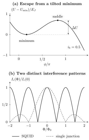
The upper panel plots $U/E_J=-\cos\phi-0.5\phi$ relative to its local minimum and marks the local minimum, saddle and forward barrier. The lower panel contrasts the normalized uniform-junction Fraunhofer envelope with the symmetric, negligible-inductance SQUID envelope. The horizontal variable is the effective flux for each different geometry; equal normalized flux does not imply equal applied field.

The local undamped plasma frequency is

$$\begin{aligned} \omega_{p0}&=\sqrt{\frac{2eI_c}{\hbar C}},\\ \omega_p(i_b)&=\omega_{p0}(1-i_b^2)^{1/4}. \end{aligned}$$

When underdamped, linearized motion has decay rate $1/(2RC)$ and oscillation frequency $\sqrt{\omega_p^2-(2RC)^{-2}}$. Beyond that regime the two relaxation rates are real, and there is no local oscillation. At zero bias the damping ratio can be expressed through

$$\beta_c=\frac{2eI_cR^2C}{\hbar}=(\omega_{p0}RC)^2.$$

Large $\beta_c$ allows inertia and hysteresis; the precise response also depends on bias and noise. In the noiseless $C=0$ limit, averaging a complete phase traversal gives

$$\langle V\rangle=R\,\operatorname{sgn}(I_b) \sqrt{I_b^2-I_c^2},\qquad |I_b|>I_c.$$

Below threshold the deterministic stationary branch has zero voltage. Rounding and premature switching require more than this elementary model.

SQUID interference

A dc SQUID has two junctions in a loop. Neglect loop inductance and choose an orientation with $\phi_1-\phi_2=2\pi\Phi_{\rm ext}/\Phi_0$ modulo $2\pi$. For critical currents $I_1,I_2>0$, maximizing their summed sinusoids gives

$$I_{c,\rm SQ}^2=I_1^2+I_2^2 +2I_1I_2\cos(2\pi\Phi_{\rm ext}/\Phi_0).$$

Thus the maximum is $I_1+I_2$ and the half-flux minimum is $|I_1-I_2|$. Identical junctions give $2I_1|\cos(\pi\Phi_{\rm ext}/\Phi_0)|$. Unlike the single-junction Fraunhofer envelope, this ideal modulation repeats without decaying lobes.

Finite loop inductance requires self-consistency between circulating current, phase and total flux $\Phi=\Phi_{\rm ext}+LI_{\rm circ}$. A SQUID detects flux coupled to its loop through a bias-dependent transfer function. Its field sensitivity additionally depends on effective area, geometry and flux noise.

From a junction to a quantum circuit

For a simple superconducting island, a chosen integer pair-number coordinate $n$ and its compact phase give

$$\begin{aligned} H&=4E_C(n-n_g)^2-E_J\cos\phi,\\ E_C&=\frac{e^2}{2C_\Sigma}. \end{aligned}$$

The globally well-defined operator statement is $[n,e^{i\phi}]=e^{i\phi}$: the exponential shifts the integer charge coordinate. Writing $[\phi,n]=i$ is a useful local phase representation, but a globally periodic angle is not an ordinary unbounded canonical position operator. The orientation of $n$ must match the chosen phase and island charge.

Capacitance supplies a dynamical charge degree of freedom, while the cosine supplies inductance and anharmonicity. The detailed quantization, control and readout are developed in Circuit QED; the superconducting-qubit page connects the circuit to processor architectures.

Exercises

1. Recover the channel tunnel limit

Use the short-channel spectrum to recover the zero-temperature tunnel-limit $I_cR_N$ for $\tau\ll1$, taking $G_N=2e^2\tau/h$ for one spin-degenerate channel.

Solution

To leading order $E_A\simeq\Delta$, so $I_c=e\Delta\tau/(2\hbar)$. Multiplication by $R_N=h/(2e^2\tau)$ gives $I_cR_N=\pi\Delta/(2e)$. The cancellation of transparency relies on the same channel and low-transmission approximation in both measurements.

2. Switching before the critical current

Find the forward barrier at $I_b=0.5I_c$ and $0.9I_c$. Derive its scaling as $I_b\to I_c^-$.

Solution

Evaluating the displayed potential difference gives $\Delta U/E_J\simeq0.68485$ and $0.05993$, respectively. Let $\epsilon=1-i_b$. Expansion near the merging minimum and saddle gives

$$\Delta U\simeq\frac{4\sqrt2}{3}E_J\epsilon^{3/2}.$$

The barrier can become comparable to thermal fluctuations while a local minimum still exists. Predicting a switching distribution also requires an escape prefactor, damping and ramp rate; barrier height alone is insufficient.

3. Average a running phase

Derive the noiseless overdamped current–voltage relation for $I_b>I_c$.

Solution

The traversal time is

$$\begin{aligned} T_\phi&=\frac{\hbar}{2eR}\int_0^{2\pi} \frac{d\phi}{I_b-I_c\sin\phi},\\ &=\frac{\hbar}{2eR}\frac{2\pi}{\sqrt{I_b^2-I_c^2}}. \end{aligned}$$

Multiplying $2\pi/T_\phi$ by $\hbar/(2e)$ gives $\langle V\rangle=R\sqrt{I_b^2-I_c^2}$. Negative bias reverses its sign. The averaging weights slow portions of the phase trajectory more strongly; simply averaging $\sin\phi$ uniformly would miss the result.

4. Compare two magnetic patterns

A uniform single junction has successive positive-field zeros separated by $0.80\,\mathrm{mT}$. A negligible-inductance SQUID has maximum and minimum currents $3.0$ and $0.6\,\mu\mathrm A$. Infer the effective junction area and the two SQUID critical currents.

Solution

The junction area is $A_{\rm eff}=\Phi_0/\Delta B\simeq2.58\,\mu\mathrm m^2$. The zeros on opposite sides of its central lobe are instead separated by $2\Phi_0/A_{\rm eff}$.

For the SQUID, $I_1+I_2=3.0\,\mu\mathrm A$ and $|I_1-I_2|=0.6\,\mu\mathrm A$, giving $1.8$ and $1.2\,\mu\mathrm A$. These inferences assume sinusoidal junctions, negligible loop inductance and controlled magnetic geometry.

References

• V. Ambegaokar and A. Baratoff, “Tunneling Between Superconductors,” Physical Review Letters 10, 486–489 (1963), doi:10.1103/PhysRevLett.10.486; correction, Physical Review Letters 11, 104 (1963), doi:10.1103/PhysRevLett.11.104.
• A. Barone and G. Paternò, Physics and Applications of the Josephson Effect, Wiley (1982), doi:10.1002/352760278X.
• A. Blais, A. L. Grimsmo, S. M. Girvin, and A. Wallraff, “Circuit Quantum Electrodynamics,” Reviews of Modern Physics 93, 025005 (2021), doi:10.1103/RevModPhys.93.025005.
• Bureau International des Poids et Mesures, “Mise en pratique for the definition of the ampere and other electric units in the SI,” SI Brochure, 9th ed., Appendix 2 (20 May 2019), §4, official BIPM appendix.
• A. A. Golubov, M. Yu. Kupriyanov, and E. Il’ichev, “The Current–Phase Relation in Josephson Junctions,” Reviews of Modern Physics 76, 411–469 (2004), doi:10.1103/RevModPhys.76.411.
• B. D. Josephson, “Possible New Effects in Superconductive Tunnelling,” Physics Letters 1, 251–253 (1962), doi:10.1016/0031-9163(62)91369-0.
• R. L. Kautz, “Noise, Chaos, and the Josephson Voltage Standard,” Reports on Progress in Physics 59, 935–992 (1996), doi:10.1088/0034-4885/59/8/001.
• D. E. McCumber, “Effect of ac Impedance on dc Voltage–Current Characteristics of Superconductor Weak-Link Junctions,” Journal of Applied Physics 39, 3113–3118 (1968), doi:10.1063/1.1656743.
• S. Shapiro, “Josephson Currents in Superconducting Tunneling: The Effect of Microwaves and Other Observations,” Physical Review Letters 11, 80–82 (1963), doi:10.1103/PhysRevLett.11.80.
• W. C. Stewart, “Current–Voltage Characteristics of Josephson Junctions,” Applied Physics Letters 12, 277–280 (1968), doi:10.1063/1.1651991.