Superconducting Proximity Effect

A superconducting contact can induce pair correlations in a material with no local attractive interaction. The same contact can weaken the parent superconductor. These direct and inverse proximity effects are two parts of a spatially coupled problem, and neither is summarized by a single fitted gap.

We develop equilibrium correlations, interface matching and spectra in clean and diffusive heterostructures. The main distinction is between a pair correlator, a self-consistent pair potential and a spectral gap. Proximity and Andreev Physics treats individual interface-conversion events and discrete hybrid levels; Josephson physics explains the resulting phase current and circuit dynamics.

Required background. BCS Theory supplies the homogeneous paired state; Green Functions in Many-Body QM supplies correlators and spectra. Helpful background. Thermal Green Functions explains Matsubara sums, while Boltzmann Transport explains elastic scattering and diffusion.

Pair correlations, pair potential and spectral gap

Use inverse-energy imaginary time $\vartheta\in[0,\beta)$, with $\beta=1/(k_BT)$, and define

$$F_{\alpha\beta}(1,2)=-\langle\mathcal T_\vartheta \psi_\alpha(1)\psi_\beta(2)\rangle.$$

The fermionic Matsubara energies are $\varepsilon_n=(2n+1)\pi k_BT$, rather than angular frequencies. Thus

$$\begin{aligned} F(i\varepsilon_n)&=\int_0^\beta d\vartheta\, e^{i\varepsilon_n\vartheta}F(\vartheta),\\ F(\vartheta)&=k_BT\sum_n e^{-i\varepsilon_n\vartheta}F(i\varepsilon_n). \end{aligned}$$

For a local attractive singlet interaction $g_{\rm pair}>0$, choose the BCS convention

$$\Delta=g_{\rm pair}\langle\psi_\downarrow\psi_\uparrow\rangle =g_{\rm pair}F_{\uparrow\downarrow}(0^-).$$

The interaction, momentum measure and cutoff determine the units and magnitude of $\Delta$. If the retained interaction is zero in a normal layer, then $\Delta_N=0$ there even though $F_N\neq0$: correlations arrive from the neighboring superconductor. A nonzero $F_N$ alone establishes neither an independent ordered phase nor a hard spectral gap.

A minigap instead means an interval with no spectral states in a specified retarded boundary-value problem. The local density of states, a minimum BdG eigenenergy and a thermally broadened tunneling threshold need not coincide. A state can have negligible weight at one probe position, and a finite-temperature conductance can be nonzero inside a true spectral gap.

Choosing a spatial description

Let $\ell=v_F\tau$ be the elastic mean free path and $d$ a layer thickness. For an approximately isotropic three-dimensional metal, $D=v_F^2\tau/3$; another dimension or Fermi surface changes that relation. The diffusion energy is

$$E_{\rm Th}=\frac{\hbar D}{d^2}.$$

This is a propagation scale, not automatically a gap. A controlled hierarchy matters more than whether a sample is casually called clean or dirty.

Description	Useful regime
Microscopic Gor’kov or BdG equations	atomic reconstruction, few modes or no separation from the Fermi scale
Eilenberger equation	energies and self-energies small relative to $E_F$, envelopes slow relative to $k_F^{-1}$; trajectories retained
Usadel equation	momentum nearly isotropic after elastic scattering; $\ell$ shorter than relevant spatial scales
Ginzburg–Landau theory	static long-wavelength amplitudes near a continuous transition

For the diffusive limit, the retained low energies should be well below $\hbar/\tau$, itself well below $E_F$. A useful spatial check is $\ell/L\ll1$ for each resolved variation length $L$. This hierarchy applies to the low-energy description; a renormalized gap equation handles its high-energy tail separately. Large resistivity alone is insufficient, especially near localization. Eilenberger theory can include impurity self-energies without taking the isotropic limit.

Quasiclassical propagator and Nambu convention

To keep the scalar diffusive equations real on positive Matsubara energies, use the phase-rotated spinor

$$\Psi=(\psi_\uparrow,i\psi_\downarrow^\dagger)^{\mathsf T}, \qquad \widehat G=-\langle\mathcal T_\vartheta\Psi\Psi^\dagger\rangle.$$

In this basis $F_{\uparrow\downarrow}=i\widehat G_{12}$. With $\tau_i$ the Nambu Pauli matrices, the uniform inverse propagator is

$$\widehat G^{-1}=i\varepsilon_n\tau_0-\xi\tau_3 +\operatorname{Im}\Delta\,\tau_1 +\operatorname{Re}\Delta\,\tau_2.$$

For real $\Delta$, $\widehat G_{12}=-i\Delta/(\varepsilon_n^2+\xi^2+\Delta^2)$, so the physical anomalous function is positive $\Delta/(\varepsilon_n^2+\xi^2+\Delta^2)$ in this convention. Rotating the spinor without rotating the gap matrix would change signs incorrectly.

Integrate across the narrow Fermi-energy coordinate, while retaining the position and Fermi-surface direction:

$$\widehat g=\frac{i}{\pi}\int d\xi\,\tau_3\widehat G, \qquad \widehat g^2=1.$$

The integration eliminates rapid microscopic oscillations and leaves slow envelopes. Some references normalize the propagator to square to $-\pi^2$ instead; their factors must be converted before use. For a uniform real singlet gap,

$$\widehat g_{\rm bulk}= \frac{\varepsilon_n\tau_3+\Delta\tau_1} {\sqrt{\varepsilon_n^2+\Delta^2}}.$$

This example checks both the phase rotation and normalization. A bare Wigner transform uses a fixed gauge; a gauge-covariant transform needs links between its field points. With electron charge $q_e=-e$, define

$$\mathcal D\widehat X=\nabla\widehat X -\frac{iq_e}{\hbar}[\tau_3\mathbf A,\widehat X].$$

The Eilenberger equation in this normalization is

$$\hbar\mathbf v_F\cdot\mathcal D\widehat g +[\widehat\Omega_n,\widehat g]=0,$$

where

$$\widehat\Omega_n=\varepsilon_n\tau_3 +\operatorname{Re}\Delta\,\tau_1 -\operatorname{Im}\Delta\,\tau_2+\widehat\Sigma_n.$$

$\widehat\Sigma_n$ contains compatible self-energies. For example, isotropic elastic scattering contributes $\hbar\langle\widehat g\rangle/(2\tau)$ in the simple nonmagnetic Born approximation. Spin, band and nonequilibrium extensions require a larger matrix structure.

Ballistic and diffusive decay

In a weakly correlated normal region, at $\varepsilon_n>0$ and $\mathbf A=0$, the anomalous component on an outgoing trajectory satisfies

$$\hbar v_{Fx}\partial_x f+2\varepsilon_n f=0.$$

Thus $f(x)=f(0)e^{-2\varepsilon_n x/(\hbar v_{Fx})}$ for $v_{Fx}>0$. The lowest Matsubara component has thermal propagation length $\hbar|v_{Fx}|/(2\pi k_BT)$. Angular averaging, grazing trajectories and boundary scattering prevent this from being one universal ballistic coherence length.

After strong elastic isotropization, the matrix Usadel equation is

$$\hbar D\mathcal D(\widehat g\mathcal D\widehat g) -[\widehat\Omega_n,\widehat g]=0.$$

For a one-dimensional spin-inactive singlet, real $\Delta$, zero phase gradient and $\mathbf A=0$, write

$$\widehat g_n=\tau_3\cos\theta_n+\tau_1\sin\theta_n.$$

Normalization is now automatic. Substitution gives

$$\frac{\hbar D}{2}\theta_n'' =\varepsilon_n\sin\theta_n-\Delta\cos\theta_n.$$

The uniform solution has $\tan\theta_n=\Delta/\varepsilon_n$. In a weakly correlated normal layer, $\Delta=0$ and $|\theta_n|\ll1$, so

$$\begin{aligned} \theta_n''&=\theta_n/\xi_n^2,\\ \xi_n&=\sqrt{\frac{\hbar D}{2\varepsilon_n}}. \end{aligned}$$

The semi-infinite decaying solution is exponential. At $D=3.0\times10^{-3}\,\mathrm{m^2s^{-1}}$ and $T=2.40\,\mathrm K$, the lowest-component length is $39.0\,\mathrm{nm}$; propagation through $30\,\mathrm{nm}$ reduces it by a factor $0.463$. This is one Matsubara component, not the full retarded spectrum. Zero-temperature spatial tails can be algebraic after the low-energy contributions are combined.

Interface matching and a finite normal film

Let $x$ increase from material 1 into material 2. For a spin-inactive tunnel interface, the Kupriyanov–Lukichev condition is

$$\sigma_1\theta_1'=\sigma_2\theta_2' =G_B\sin(\theta_2-\theta_1),$$

where $\sigma_i$ are normal conductivities and $G_B$ is conductance per area. Matrix form replaces the last member by $(G_B/2)[\widehat g_1,\widehat g_2]$ and the left members by $\sigma_i\widehat g_i\partial_x\widehat g_i$. Using outward normals on both materials reverses one derivative sign.

The weighted matrix current matches across this interface. Neither $\theta$ nor its bare derivative is generally continuous. This does not say the whole matrix current is spatially constant inside each material: the commutator in the transport equation acts as a source for its nonconserved components. Charge conservation follows the appropriate projection and self-consistency. A magnetic interface can exchange spin torque, so full spin-current continuity is not generally valid.

For an explicit solvable example, let a rigid reservoir with small angle $\theta_S$ contact a normal film $0<x<d$. The free outer surface reflects quasiparticles, giving $\theta_N'(d)=0$. Linearizing the tunnel boundary condition gives

$$\sigma_N\theta_N'(0)=G_B[\theta_N(0)-\theta_S].$$

Define $\gamma_B=\sigma_N/(G_B\xi_n)$ and $b=d/\xi_n$. The solution is

$$\frac{\theta_N(x)}{\theta_S} =\frac{\cosh[(d-x)/\xi_n]} {\cosh b+\gamma_B\sinh b}.$$

The reflecting surface flattens the profile instead of absorbing correlations. Increasing interface resistance increases $\gamma_B$ and suppresses the amplitude. In the semi-infinite limit,

$$\frac{\theta_N(x)}{\theta_S} \longrightarrow\frac{e^{-x/\xi_n}}{1+\gamma_B}.$$

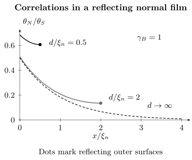
Exact linearized profiles for $\gamma_B=1$. The finite curves stop at reflecting surfaces $d/\xi_n=0.5$ and 2, where their slopes vanish. The dashed semi-infinite curve continues to decay. The vertical quantity is a small Matsubara angle normalized to the reservoir value, not an energy gap or a superconducting fraction.

A low total conductance does not by itself prove that every channel is a tunnel channel. Arbitrary transmissions require an appropriate Nazarov or scattering-matrix boundary condition. Spin mixing, filtering and orbital reconstruction require additional information, including phases that ordinary normal-state conductance does not determine. Near $T_c$, linearization can simplify these conditions; at low temperature the full transmission distribution can matter.

Inverse proximity and self-consistency

A rigid reservoir fixes the parent propagator and excludes its suppression by construction. To calculate inverse proximity, solve both layers together and determine the parent pair potential self-consistently.

For a local isotropic singlet channel with isolated transition temperature $T_{c0}$, one regularized form is

$$0={}\Delta(x)\ln\frac{T}{T_{c0}} +2\pi k_BT\sum_{n\geq0} \left[\frac{\Delta(x)}{\varepsilon_n}-f_s(x,\varepsilon_n)\right].$$

Here $f_s=\sin\theta_n$ in the diffusive real-gap case; a trajectory calculation uses its angular average. The positive-energy factor two, pairing convention and cutoff elimination are part of this equation. In a layer with no local attraction, set $\Delta=0$ instead of assigning it a fictitious $T_{c0}$.

Near a mean-field transition, linearized transport plus this equation gives a global eigenvalue problem for the stack. An arbitrary local $T_c(x)$ is not a substitute. A resistive midpoint need not equal that mean-field instability, especially when fluctuations, inhomogeneity or percolating paths matter.

For a numerical calculation, start from a trial $\Delta(x)$, solve the normalized Matsubara boundary problem, update the gap equation and iterate. Check the spatial mesh, Matsubara tail and interface residuals independently. Then solve the retarded problem with the converged $\Delta(x)$; convergence of the transition eigenproblem alone does not establish low-temperature spectral convergence. Damage, interdiffusion and changed band structure or interactions can also reduce $T_c$, so thickness trends should be compared with structural and normal-state measurements.

Retarded spectra and the role of geometry

In the scalar convention,

$$\frac{N(E,x)}{N_0}=\operatorname{Re}\cos\theta^R(E,x).$$

$N_0$ and $N$ must use the same spin convention. Continue $\varepsilon_n\to-i(E+i0^+)$ on the physical analytic branch; do not independently choose square-root signs at each energy. A positive Matsubara amplitude is not enough to infer a gap.

For a long, transparent, zero-phase diffusive SNS junction with rigid gapped reservoirs and negligible pair breaking,

$$E_g\simeq3.12\,\frac{\hbar D}{L^2}, \qquad \Delta\gg\frac{\hbar D}{L^2}.$$

$L$ is the full normal-region length. Reflection symmetry relates its half-interval to a normal film of thickness $d=L/2$ with one reflecting end. In that corresponding ideal limit the film coefficient is $3.12/4\simeq0.78$ multiplying $\hbar D/d^2$, not 3.12. An unbounded normal region has no finite hard minigap, even though its low-energy local density of states can be strongly suppressed. The SNS benchmark is discussed by Zhou et al. (1998), and the boundary distinctions by Belzig et al. (1999).

Finite interface resistance, phase difference, pair breaking and an incompletely rigid parent change the spectral problem. Temperature mainly enters the equilibrium gap and occupations; thermal or instrumental convolution further changes a measured edge without defining the underlying spectral gap. Tunneling Spectroscopy develops that distinction.

Ferromagnets and pair-symmetry conversion

Fermi antisymmetry requires

$$F_{\alpha\beta}(\mathbf R,\mathbf p,i\varepsilon_n) =-F_{\beta\alpha}(\mathbf R,-\mathbf p,-i\varepsilon_n).$$

Include orbital or band exchange labels when present. In a single-band orbital-symmetric channel, an even-parity equal-spin amplitude is therefore odd in Matsubara energy. This is a symmetry of a correlation function, not by itself a new thermodynamic phase or a topological invariant.

In a collinear diffusive ferromagnet with exchange coefficient $h$ (spin-band splitting $2h$), the linear combinations $f_\pm=f_s\pm f_{t0}$ obey, in a compatible spin convention,

$$\begin{aligned} \hbar D_F f_\pm''&=2(\varepsilon_n\pm ih)f_\pm,\\ k_\pm^2&=\frac{2(\varepsilon_n\pm ih)}{\hbar D_F}. \end{aligned}$$

Choose roots with positive real part for decay. At $h\gg\pi k_BT$, the decay and oscillation lengths approach $\xi_F=\sqrt{\hbar D_F/h}$. The scalar spin-independent angle cannot describe this conversion.

Noncollinear magnetization and suitable spin-active structures can generate equal-spin correlations perpendicular to the local exchange direction. They avoid the uniform exchange dephasing of the short-range component and can approach the thermal range $\sqrt{\hbar D_F/(2\pi k_BT)}$. Spin relaxation, texture and interface coupling still limit their propagation. Spin mixing at a purely collinear interface alone need not generate a long-range equal-spin component.

For $D_F=2.0\times10^{-4}\,\mathrm{m^2s^{-1}}$, $h=20\,\mathrm{meV}$ and $T=2.00\,\mathrm K$, the ideal short and long scales are $2.57$ and $11.0\,\mathrm{nm}$. A configuration-dependent signal persisting beyond the first length motivates a conversion model, but does not uniquely identify it. Pinholes, stray fields, heating and magnetic dead layers can also alter a signal. A zero-bias peak is not a substitute for the symmetry analysis (Bergeret et al., 2005; Eschrig, 2015).

Exercises

1. Derive the finite-film profile

Derive the displayed linearized solution with a reflecting outer surface. For $d=\xi_n$ and $\gamma_B=1$, find $\theta_N(0)/\theta_S$ and $\theta_N(d)/\theta_S$.

Solution

The zero-derivative boundary leaves $\theta_N=A\cosh[(d-x)/\xi_n]$. At the interface,

$$-\frac{\sigma_N A}{\xi_n}\sinh b =G_B(A\cosh b-\theta_S).$$

Solving for $A$ gives the stated denominator. For $b=\gamma_B=1$, the interface ratio is $\cosh1/e\simeq0.5677$ and the outer-surface ratio is $e^{-1}\simeq0.3679$. The interface jump is compatible with continuous weighted spectral current. The solution assumes small angles; it must not be used to infer the hard minigap by linearization.

2. Recover the bulk normalization

For a real uniform gap, invert the stated microscopic matrix and integrate over $\xi$ to recover $\widehat g_{\rm bulk}$.

Solution

The inverse is

$$\widehat G=-\frac{i\varepsilon_n\tau_0+\xi\tau_3-\Delta\tau_2} {\varepsilon_n^2+\xi^2+\Delta^2}.$$

The odd $\xi$ integral vanishes. Using $\tau_3\tau_2=-i\tau_1$ and $\int_{-\infty}^{\infty}d\xi/(\xi^2+a^2)=\pi/a$ gives $(\varepsilon_n\tau_3+\Delta\tau_1)/\sqrt{\varepsilon_n^2+\Delta^2}$. Anticommutation of $\tau_1$ and $\tau_3$ then gives $\widehat g^2=1$. Also $i\widehat G_{12}=\Delta/(\varepsilon_n^2+\xi^2+\Delta^2)$, checking the physical anomalous sign.

3. Distinguish two minigap geometries

For $D=10^{-2}\,\mathrm{m^2s^{-1}}$ and normal length $500\,\mathrm{nm}$, compare an ideal long zero-phase SNS junction with an SN film of that same thickness and a reflecting outer surface.

Solution

Both have $\hbar D/(500\,\mathrm{nm})^2=0.0263\,\mathrm{meV}$. The SNS benchmark is $E_g\simeq0.0821\,\mathrm{meV}$. The reflecting film corresponds to an SNS normal length $1000\,\mathrm{nm}$ and has $E_g\simeq0.0205\,\mathrm{meV}$. These require a large parent gap, transparent interfaces, diffusion and negligible pair breaking. Replacing the reflecting boundary by an open normal reservoir changes the answer again.

4. Follow the exchange modes

For $\varepsilon_n\ll h$, show that a singlet injected with $f_+(0)=f_-(0)=f_0$ has a damped oscillation, and classify an even-parity equal-spin component in the same single-band model.

Solution

The decaying roots approach $k_\pm=(1\pm i)/\xi_F$. Therefore

$$\begin{aligned} f_s(x)&=f_0e^{-x/\xi_F}\cos(x/\xi_F),\\ f_{t0}(x)&=-if_0e^{-x/\xi_F}\sin(x/\xi_F). \end{aligned}$$

The imaginary relative phase follows the displayed Matsubara convention. Equal-spin and even spatial parity are both symmetric, so the additional frequency parity must be odd. Neither that classification nor an oscillating thickness dependence alone proves a separate phase, a $\pi$ junction or topology.

References

• W. Belzig, F. K. Wilhelm, C. Bruder, G. Schön, and A. D. Zaikin, “Quasiclassical Green’s Function Approach to Mesoscopic Superconductivity,” Superlattices and Microstructures 25, 1251–1288 (1999), doi:10.1006/spmi.1999.0710.
• F. S. Bergeret, A. F. Volkov, and K. B. Efetov, “Odd Triplet Superconductivity and Related Phenomena in Superconductor–Ferromagnet Structures,” Reviews of Modern Physics 77, 1321–1373 (2005), doi:10.1103/RevModPhys.77.1321.
• A. I. Buzdin, “Proximity Effects in Superconductor–Ferromagnet Heterostructures,” Reviews of Modern Physics 77, 935–976 (2005), doi:10.1103/RevModPhys.77.935.
• G. Eilenberger, “Transformation of Gorkov’s Equation for Type II Superconductors into Transport-Like Equations,” Zeitschrift für Physik 214, 195–213 (1968), doi:10.1007/BF01379803.
• M. Eschrig, “Spin-Polarized Supercurrents for Spintronics: A Review of Current Progress,” Reports on Progress in Physics 78, 104501 (2015), doi:10.1088/0034-4885/78/10/104501.
• M. Yu. Kuprianov and V. F. Lukichev, “Influence of Boundary Transparency on the Critical Current of ‘Dirty’ SS’S Structures,” Soviet Physics JETP 67, 1163–1168 (1988).
• Yu. V. Nazarov, “Novel Circuit Theory of Andreev Reflection,” Superlattices and Microstructures 25, 1221–1231 (1999), doi:10.1006/spmi.1999.0738.
• K. D. Usadel, “Generalized Diffusion Equation for Superconducting Alloys,” Physical Review Letters 25, 507–509 (1970), doi:10.1103/PhysRevLett.25.507.
• F. Zhou, P. Charlat, B. Spivak, and B. Pannetier, “Density of States in Superconductor-Normal Metal-Superconductor Junctions,” Journal of Low Temperature Physics 110, 841–850 (1998), doi:10.1023/A:1022628927203.