Scanning Tunneling Microscopy and Spectroscopy

Scanning tunneling microscopy (STM) holds a conducting tip a few ångströms from a conducting surface and regulates the vacuum tunneling current while the tip scans. Scanning tunneling spectroscopy (STS) records the current or differential conductance as the bias is varied at a point, along a line, or across a grid. The same junction can therefore resolve atomic-scale spatial structure and millielectronvolt-scale spectral structure.

Neither output is a direct photograph of atoms or of the local density of states. The recorded current depends exponentially on tip–sample separation and also on the electronic states, tip apex, tunneling matrix element, occupation factors, feedback history, voltage modulation, and instrumental response. Atomic resolution means that the junction is sensitive to atomic-scale electronic structure; it does not make every bright maximum an atomic coordinate.

The discussion below starts with an elastic, weakly coupled junction whose electrodes remain in thermal equilibrium separately. It then explains what changes when the tip spectrum, feedback, or sample response matters.

Required background. Tunneling Applications: First Encounters supplies the exponential dependence of tunneling on barrier width. Spectral Functions supplies local transition weights, and Green Functions in Many-Body QM supplies the retarded propagator and spectral-density relation. How Quantum Matter Is Measured supplies the forward-model, calibration and resolution checks needed to interpret the tip–sample signal.

Tunneling current and local electronic spectra

The tip, vacuum gap, and sample form a voltage-biased junction. A current preamplifier measures the tunneling signal, while piezoelectric actuators move the tip. In constant-current imaging, feedback adjusts the vertical coordinate to keep the measured current near its setpoint. The recorded height therefore depends on the electronic states as well as the surface geometry.

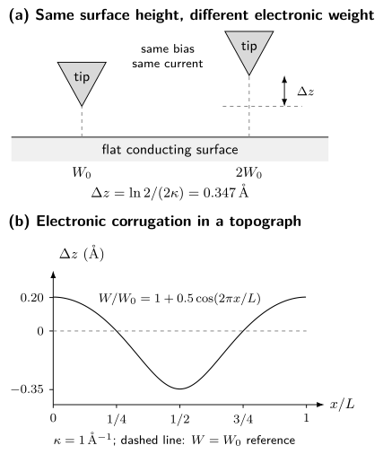
Top: at the same current and bias, doubling the integrated electronic weight requires a retraction $\Delta z=\ln 2/(2\kappa)$, even when both sites have the same geometric height. Bottom: for a flat surface with $W(x)/W_0=1+0.5\cos(2\pi x/L)$ and $\kappa=1\,\mathrm{\mathring A}^{-1}$, the apparent height relative to the $W_0$ setpoint is $\Delta z=\ln[W(x)/W_0]/(2\kappa)$. The curve is calculated from the constant-current model developed below; the junction drawing is schematic.

Bias and current convention

This page uses sample bias

$$V = V_{\mathrm{sample}} - V_{\mathrm{tip}},$$

with $e\gt0$. For a normal-metal tip in the usual elastic-tunneling convention:

• $V\gt0$ predominantly probes empty sample states between the sample Fermi level and $E_F+eV$;
• $V\lt0$ predominantly probes occupied sample states between $E_F+eV$ and the sample Fermi level.

Here $I$ is positive for net electron transfer from tip to sample, multiplied by the positive charge magnitude $e$. Conventional charge flows in the opposite direction. With this choice a normal passive junction has $I/V>0$ near zero bias. Check the instrument’s sign before using its output: laboratories use both current conventions. The simple occupied/empty assignment also needs modification for strong band bending, structured tip spectra, or large biases.

Tunneling current

Transfer-Hamiltonian expression

Bardeen’s weak-coupling construction treats tip and sample as separately equilibrated electrodes and couples their states perturbatively. For tip state $\mu$ and sample state $\nu$, the matrix element can be evaluated on a surface $S$ inside the barrier:

$$M_{\mu\nu} = -\frac{\hbar^2}{2m} \int_S d\mathbf S\cdot \left( \psi_\mu^*\nabla\psi_\nu - \psi_\nu\nabla\psi_\mu^* \right).$$

For sample bias $V$, the electrode electrochemical potentials obey $\mu_t-\mu_s=eV$. Measure $E$ from $\mu_s$, so that the same tunneling electron has energy $E-eV$ relative to the tip. For equal electrode temperatures, a useful continuum form of the elastic current is

$$I(\mathbf r_0,V) \propto \int_{-\infty}^{\infty} dE\, \times \rho_t(E-eV) \times \rho_s^{(M)} \left( \mathbf r_0,E;V \right) \times \left[ f(E-eV)-f(E) \right].$$

Here $\rho_t$ is the tip density of states and $\rho_s^{(M)}$ is a matrix-element-weighted sample spectrum. The notation deliberately avoids identifying it with the bare sample density of states. Tip orbital symmetry, lateral momentum filtering, barrier shape, surface termination, and the voltage-dependent junction geometry all enter $M_{\mu\nu}$.

The perturbative expression assumes a weak junction. At contact, at very high current, or under strong nonequilibrium drive, multiple scattering, force, heating, and atomic rearrangement invalidate the simple transfer picture.

Exponential distance sensitivity

For a locally rectangular barrier of effective height $\bar\Phi$ and low bias, a wavefunction decays with

$$\kappa \simeq \frac{\sqrt{2m\bar\Phi}}{\hbar}, \qquad I(z) \propto e^{-2\kappa z}.$$

In practical units,

$$\begin{aligned} \kappa &\simeq 0.512\, \sqrt{\frac{\bar\Phi}{\mathrm{eV}}} \ \mathrm{\mathring A}^{-1}, \\ 2\kappa &\simeq 1.025\, \sqrt{\frac{\bar\Phi}{\mathrm{eV}}} \ \mathrm{\mathring A}^{-1}. \end{aligned}$$

For $\bar\Phi=4\,\mathrm{eV}$, retracting the tip by $1\,\mathrm{\mathring A}$ reduces the idealized current by about a factor of eight. This exponential selectivity explains high vertical sensitivity and why vibration, drift, and a second microscopic protrusion on the tip are consequential.

An $I(z)$ curve can define an apparent barrier height:

$$\Phi_{\mathrm{app}} = \frac{\hbar^2}{8m} \left( \frac{\partial\ln\lvert I\rvert}{\partial z} \right)^2.$$

$\Phi_{\mathrm{app}}$ is a junction diagnostic, not automatically the arithmetic mean of independently measured work functions. Image potentials, bias, orbital character, piezo calibration, and mechanical relaxation can change the slope.

Local spectral density and the Tersoff–Hamann limit

The local single-particle spectral density is related to the retarded Green function by

$$\rho_s(\mathbf r,E) = -\frac{1}{\pi} \operatorname{Im} G_s^{\mathrm R}(\mathbf r,\mathbf r;E).$$

For independent particles this reduces to

$$\rho_s(\mathbf r,E) = \sum_n \left| \psi_n(\mathbf r) \right|^2 \delta(E-E_n).$$

Here $G_s^R$ is the energy-domain electron Green function, with energy measured from $E_F=\mu_s$ and all required physical spin components included. This LDOS contains the spatial weight of each state; a tunneling measurement may weight those components further through the junction matrix element.

Tersoff and Hamann modeled an $s$-wave tip apex and a weak, low-bias vacuum junction. At low temperature, with a featureless tip spectrum and slowly varying matrix element,

$$I(\mathbf r_0,V) \propto \int_0^{eV} d\epsilon\, \rho_s \left( \mathbf r_0, \epsilon \right),$$

and therefore

$$\frac{dI}{dV}(\mathbf r_0,V) \propto \rho_s \left( \mathbf r_0, eV \right).$$

The spectral arguments here and below are energies relative to the sample Fermi level. The position $\mathbf r_0$ is the tip center in the vacuum, where the sample wavefunctions have evanescent tails. Their distance dependence is already present in this vacuum LDOS: multiplying it by another barrier-decay factor would count that dependence twice. Below, a separate exponential is used only after factoring an approximate common decay out of a surface spectrum.

The relation between $dI/dV$ and LDOS is the central STS approximation. The proportionality can fail or become strongly weighted when:

• the tip density of states varies over the bias window;
• the apex has important $p$- or $d$-orbital character;
• several sample orbitals have different vacuum decay constants;
• the barrier transmission changes rapidly with bias;
• the sample is semiconducting and the tip electric field bends bands;
• the voltage drops outside the intended vacuum barrier;
• the junction becomes inelastic, nonequilibrium, or strongly coupled.

Chen’s derivative rule makes the orbital warning concrete: a nonspherical apex can couple to spatial derivatives of the sample wavefunction rather than simply to its value at $\mathbf r_0$. Changing the tip can then reverse contrast or suppress a state without changing the sample.

Thermal and modulation broadening

With a normal, featureless tip and bias-independent matrix element, finite temperature gives approximately

$$\frac{dI}{dV}(V) \propto \int_{-\infty}^{\infty} dE\, \rho_s(E) \times \left[ -\frac{\partial f(E-eV)}{\partial E} \right].$$

The full width at half maximum of $-\partial f/\partial E$ is about $3.53k_{\mathrm B}T$. At $4.2\,\mathrm K$, this thermal width is approximately $1.28\,\mathrm{meV}$ before electrical noise or lock-in broadening is included.

A lock-in amplifier measures a first harmonic, not an infinitesimal derivative. Let the applied bias be $V+a\cos\theta$, with peak amplitude $a$ and root-mean-square amplitude $V_{\rm rms}=a/\sqrt2$. For a quasistatic junction, feedback disabled, and a correctly phased detector calibrated to return the conductance of a linear resistor, the output is

$$G_a(V)=\frac{1}{\pi a}\int_0^{2\pi} I(V+a\cos\theta)\cos\theta\,d\theta.$$

Integrating by parts changes this to an average of the true differential conductance $G_0=dI/dV$:

$$\begin{aligned} G_a(V)&=\int_{-a}^{a}K_a(v)G_0(V+v)\,dv,\\ K_a(v)&=\frac{2}{\pi a^2}\sqrt{a^2-v^2},\qquad |v|\le a, \end{aligned}$$

with $K_a=0$ outside this interval and $\int K_a(v)\,dv=1$. The kernel has energy FWHM $\sqrt3\,ea=\sqrt6\,eV_{\rm rms}$. It is not Gaussian, so its FWHM and the thermal FWHM cannot in general be combined exactly by adding their squares. Convolve the model with both kernels instead.

These formulas describe the settled, in-phase signal. A rapid voltage sweep, capacitive current, a wrong phase, or a filter that has not settled needs an additional time-dependent instrument model. The lock-in time constant alone is not a universal energy-resolution width.

Topography versus spectroscopy

Constant-current imaging

Let $h(\mathbf r)$ be the geometric surface height and $z_{\mathrm p}(\mathbf r)$ the laboratory piezo coordinate. For this model take $V_{\rm set}>0$, $I_{\rm set}>0$, and a position-independent decay constant $\kappa$. Factor the vacuum decay out of an effective surface spectrum and call its integrated weight $W$. At low temperature and bias,

$$\begin{aligned} I_{\mathrm{set}} \simeq C\, \exp \left[ -2\kappa \left( z_{\mathrm p}-h \right) \right] W(\mathbf r,V_{\mathrm{set}}), \\ W(\mathbf r,V_{\mathrm{set}}) = \int_0^{eV_{\mathrm{set}}} d\epsilon\, \rho_s \left( \mathbf r, \epsilon \right). \end{aligned}$$

Solving for the recorded piezo coordinate gives

$$z_{\mathrm p}(\mathbf r) = h(\mathbf r) + \frac{1}{2\kappa} \ln \left[ \frac{C\,W(\mathbf r,V_{\mathrm{set}})} {I_{\mathrm{set}}} \right].$$

Thus a topograph combines geometric height and integrated electronic weight. For negative setpoints, use the positive magnitude of the occupied-state integral and $|I_{\rm set}|$ in this logarithm. Spatially varying decay constants or apex orbitals need a richer model. Bias-dependent contrast can help identify electronic contributions, provided the tip and feedback response remain stable.

The feedback bandwidth must be fast enough to track the intended corrugation and slow enough not to chase current noise. Excessive gain produces ringing; insufficient gain produces tracking error. Trace and retrace disagreement can expose drift, creep, tip changes, or an unstable loop.

Constant-height imaging

With feedback disabled, the tip follows a prescribed plane and the current is recorded. Constant-height mode avoids feedback convolution and can be faster, but it is less tolerant of tilt, steps, debris, drift, and piezo nonlinearity. A collision can alter both tip and sample. Constant-height data are meaningful only when the scan plane and safety margin are documented.

Point, line, and grid spectroscopy

A common spectroscopy cycle is:

1. stabilize the feedback at $(V_{\mathrm{set}},I_{\mathrm{set}})$;
2. wait for the junction and filters to settle;
3. open the feedback loop;
4. sweep $V$ while recording $I(V)$ and optionally lock-in $dI/dV$;
5. return to the setpoint, close feedback, and move to the next position.

The derivative here is taken at fixed tip position. If the height changes during the sweep, the numerical derivative also contains $(\partial I/\partial z)(dz/dV)$. A fast modulation can measure the fixed-height response while a slower controller moves the tip, but then different bias points refer to different junction heights and need a corresponding correction. Feenstra and collaborators’ acquisition study shows how this distinction enters semiconductor spectroscopy.

The stabilization step imprints a setpoint effect. In the simple model, the fixed junction height obeys

$$e^{-2\kappa z(\mathbf r)} \propto \frac{I_{\mathrm{set}}} {W(\mathbf r,V_{\mathrm{set}})}.$$

Consequently, a conductance map scales approximately as

$$\frac{dI}{dV}(\mathbf r,V) \propto \frac{ I_{\mathrm{set}}\, \rho_s(\mathbf r,eV) }{ \displaystyle \int_0^{eV_{\mathrm{set}}} d\epsilon\, \rho_s(\mathbf r,\epsilon) }.$$

Spatial variation in the integrated denominator can create, suppress, or mix Fourier components. Comparing maps acquired with different setpoints, analyzing the simultaneously acquired current, and forward-modeling the normalization are stronger than assuming the denominator is uniform.

The normalized conductance

$$\frac{dI/dV}{I/V}$$

can reduce a slowly varying transmission factor, especially in semiconductor spectroscopy. It divides the local spectral weight by an energy-averaged weight, so it can shift or reshape a peak; it is not the LDOS itself. For an ideal metal with $I(V)=G_0V+O(V^2)$ and $G_0\ne0$, the zero-bias limit is finite and equals one. Numerical division is nevertheless sensitive to current noise and offsets near zero, and can become ill-conditioned inside a gap. Any smoothing or regularization must be included when interpreting the result.

Quasiparticle interference

An elastic defect can scatter a quasiparticle from $\mathbf k$ to $\mathbf k+\mathbf q$. Interference between incident and scattered amplitudes modulates the local spectral density. A conductance map

$$g(\mathbf r,E) \equiv \left. \frac{dI}{dV}(\mathbf r,V) \right|_{eV=E}$$

can be drift-corrected, windowed, Fourier transformed, and compared across energy to obtain dispersing features in $g(\mathbf q,E)$.

A joint-density-of-states construction,

$$J(\mathbf q,E) = \int \frac{d^d k}{(2\pi)^d}\, A(\mathbf k,E) A(\mathbf k+\mathbf q,E),$$

identifies pairs of high-spectral-weight states separated by $\mathbf q$. It is a phase-space guide, not a complete QPI theory. Define the spatial Fourier transform by

$$\delta\rho(\mathbf q,E) = \int d^d r\, e^{-i\mathbf q\cdot\mathbf r} \delta\rho(\mathbf r,E).$$

In a single-impurity $T$-matrix treatment, first form the retarded correction

$$\Lambda(\mathbf q,E) = \int \frac{d^d k}{(2\pi)^d} \operatorname{Tr} \big[ P_e G_0^R(\mathbf k+\mathbf q,E) \times T_{\mathbf k+\mathbf q,\mathbf k}^R(E) \times G_0^R(\mathbf k,E) \big].$$

Here $P_e$ projects onto all physical electron spin and orbital sectors in the declared basis. It is the identity for an electron-only basis; in a Nambu basis it excludes the duplicated hole sector. A reduced Nambu block must instead reconstruct the missing physical electron sectors with the appropriate reflected-energy hole contribution. Taking the full Nambu trace at the same energy does not give the electron LDOS.

Since the real-space LDOS is $-\operatorname{Im}G^R_{ee}(\mathbf r,\mathbf r;E)/\pi$, its Fourier correction is

$$\delta\rho(\mathbf q,E) = -\frac{ \Lambda(\mathbf q,E) -\Lambda^*(-\mathbf q,E) }{2\pi i}.$$

This form obeys $\delta\rho(-\mathbf q,E)=\delta\rho(\mathbf q,E)^*$. It retains the phase $e^{-i\mathbf q\cdot\mathbf r_0}$ of a defect displaced to $\mathbf r_0$. Replacing it by $-\operatorname{Im}\Lambda(\mathbf q,E)/\pi$ requires additional symmetry and origin choices; taking an imaginary part does not generally commute with spatial Fourier transformation. Wang and Lee’s Eq. (1) gives the conjugate-wavevector and reflected-energy structure in a superconducting Nambu representation.

The Green functions carry band, orbital, spin, particle–hole, and coherence-factor structure; the impurity $T$ matrix carries the defect potential and scattering channel. Two geometrically allowed vectors can therefore have very different intensities.

Start with the unsymmetrized real-space map: identify defects, step edges, drift, and scan-line structure before Fourier transformation. Windowing changes peak shapes; symmetry averaging can impose a symmetry that the original image does not have. Compare several energies and candidate scattering matrices, and use ARPES to constrain the band dispersion when available.

For an isotropic contour, backscattering gives $q\simeq2k$, but that mnemonic is not universal. Multiband, anisotropic, spin-textured, and superconducting systems require vector assignments and coherence factors. Absence of a nominal $2k$ peak is not by itself proof of topological protection: tip and orbital matrix elements, the impurity population, finite field of view, overlapping features, and signal-to-noise can all hide it. See Edge and Surface States for the symmetry assumptions behind forbidden backscattering.

Setpoint normalization is especially important in Fourier analysis because the denominator can mix spatial structure from the entire stabilization window into every energy slice. A Fourier peak first establishes a modulation. Dispersion can support a QPI assignment, but some scattering vectors vary too weakly to resolve over the measured energy range. Lack of visible dispersion alone proves neither static order nor the absence of QPI.

Superconducting gap imaging

With a normal tip and a simple isotropic superconductor, low-temperature conductance can show suppressed subgap weight and coherence peaks near $\lvert eV\rvert=\Delta$. Real spectra can instead reflect an anisotropic or nodal gap, several bands, pair breaking, lifetime effects, spatial inhomogeneity, surface states, competing order, and instrumental convolution. BCS Theory gives the ideal density of states and the commonly used Dynes broadening; this page focuses on what a map establishes.

For a normal, featureless tip and bias-independent transmission, fit each spectrum with the same broadened sample model:

$$\begin{aligned} g_{\mathrm{meas}}(\mathbf r,V) &= \left( \mathcal R_E * g_{\mathrm{junction}} \right) \left( \mathbf r,V \right). \end{aligned}$$

Here $g_{\mathrm{junction}}$ carries parameters such as $\Delta$ and $\Gamma$, while $\mathcal R_E$ includes thermal, modulation, and electrical resolution. Fit parameters, bounds, background, rejected pixels, covariance, and residuals should accompany the map. Half the coherence-peak separation is a descriptive energy scale, not a universal estimator of the order parameter.

With a superconducting tip, return to the tunneling-current integral and differentiate the complete result: the voltage dependence of $\rho_t(E-eV)$ contributes too. It cannot generally be replaced by the normal-tip thermal convolution above. For ideal fully gapped electrodes at zero temperature, single-quasiparticle current starts at

$$\lvert eV\rvert \simeq \Delta_t+\Delta_s,$$

not at the sample gap alone. Thermal quasiparticles can produce additional features near the difference of the gap magnitudes, and broadening softens the threshold. A sharp, calibrated tip spectrum can improve sensitivity to narrow sample features, but extraction of the sample spectrum still requires both electrodes and possible Josephson or nonequilibrium contributions.

Useful superconducting imaging modes include:

• maps of fitted gap scale, broadening, zero-bias conductance, and coherence-peak weight;
• field-dependent vortex imaging and vortex-core spectroscopy;
• impurity-bound-state maps and their particle–hole structure;
• energy-resolved QPI with superconducting coherence factors;
• Josephson STM, where pair tunneling probes local phase-coherent response.

A local single-particle gap is not automatically a superconducting order parameter. Temperature and field evolution, phase-sensitive information, vortex response, and bulk thermodynamic or electrodynamic evidence strengthen the assignment. Spatial anticorrelation between two fitted quantities does not establish that one causes the other; setpoint, fit covariance, and shared normalization must be tested.

Atomic manipulation and defects

The tip is an actuator as well as a detector. By reducing the separation, changing the bias, or applying a controlled pulse, an experiment can:

• drag, push, or pull an adsorbate laterally;
• transfer an atom or molecule between tip and sample;
• change a molecular conformation, charge state, or spin state;
• desorb material, create a vacancy, or move a domain wall;
• assemble artificial lattices, corrals, and coupled impurity structures.

Eigler and Schweizer’s low-temperature positioning of individual xenon atoms demonstrated deterministic lateral manipulation. Crommie, Lutz, and Eigler then assembled iron-atom corrals and observed confined surface-state resonances. The manipulation mechanism is junction dependent: manipulation can be driven by tip–adsorbate forces, electric fields, current-induced excitation, local heating, or chemical transfer, depending on junction parameters.

Reimage the sample and a reference region after a manipulation pulse. An apparent disappearance may mean transfer to the tip, diffusion outside the image, a changed charge state, or changed contrast. A changed apex can alter every later spectrum.

Defects can be studied rather than moved. A point defect may produce a local resonance, Friedel oscillations, a magnetic or superconducting bound state, or a charging feature. Assignment requires comparison among defect species, spatial decay and symmetry, field and temperature response, and a microscopic impurity model. The topographic shape alone rarely identifies the chemical species.

Inelastic STS detects thresholds where tunneling electrons excite a vibration, spin transition, or other local mode. The signal may appear in $d^2I/dV^2$ or as steps in $dI/dV$. Heating, vibrational pumping, and competing elastic structure must be excluded. This is a different operator channel from the elastic local spectral density.

Tip-induced perturbations

The same local electric field and force that enable manipulation can perturb passive spectroscopy:

• semiconductors and low-density systems can exhibit tip-induced band bending;
• small islands and molecules can charge, gate, or undergo Coulomb blockade;
• a magnetic or superconducting tip can exchange-couple or proximity-couple to the sample;
• high current can heat, switch, or damage the surface;
• the apex can pick up atoms and change orbital or spin sensitivity.

Varying tip height and setpoint is therefore a physical control experiment. A feature that shifts with junction resistance may belong to the junction rather than to the unperturbed sample.

Recognizing instrumental structure

Calibrate lateral distances against known lattice vectors, vertical motion with appropriate displacement standards, and voltage/current gains against electrical references. Check polarity and offsets on a known spectrum. For each map retain the bias, current setpoint, modulation amplitude and its peak/RMS convention, temperature, scan direction, feedback error, and timing. Trace/retrace and before/after spectra help reveal changes during acquisition.

Drift correction and line flattening can alter long-wavelength structure. Compare processed images with the originals, especially before attributing a Fourier peak or broken symmetry to the sample.

Symptoms and checks

Symptom	Plausible cause	Diagnostic
duplicated atoms or parallel features	double or multiple tip apex	image an isolated defect or step; recondition tip
streaks and abrupt contrast changes	tip rearrangement, feedback transient, vibration	compare trace/retrace, error channel, and time order
scan-direction-dependent lattice	creep, hysteresis, cross-coupling	rotate scan, reverse direction, calibrate both axes
broad or shifted spectral feature	temperature, modulation, voltage offset, tip spectrum	reference spectrum and full resolution convolution
spatial contrast changes with setpoint	integrated-density normalization or barrier weighting	repeat several $(V_{\mathrm{set}},I_{\mathrm{set}})$ pairs
strong low-frequency stripes	line noise, drift, feedback gain, flattening	inspect raw lines, noise spectrum, and scan-speed scaling
feature moves with junction resistance	band bending, charging, heating, force	vary tip height at fixed location and model electrostatics
Fourier peak appears after symmetrization	processing or finite-window artifact	show unsymmetrized maps and alternate windows
gap map follows topography	setpoint, tip change, or fit covariance	compare raw spectra, residuals, and independent setpoints
atom changes identity after a pulse	tip pickup or charge-state contrast	reimage reference surface and characterize the apex

Small fit uncertainties do not account for an unknown tip spectrum, spatially varying barrier, surface termination, or an incorrect scattering model. Repeated pixels from one acquisition share these uncertainties. Repeating the measurement with different tips, preparations, and setpoints tests whether the interpretation survives a changed junction.

Exercises

Exercise 1: Current–distance sensitivity

Take an effective barrier height $\bar\Phi=4.0\,\mathrm{eV}$. Estimate $\kappa$ and the current ratio $I(z+1\,\mathrm{\mathring A})/I(z)$ in the rectangular-barrier approximation.

Solution

The inverse decay length is

$$\kappa \simeq 0.512\sqrt{4.0}\, \mathrm{\mathring A}^{-1} = 1.024\, \mathrm{\mathring A}^{-1}.$$

Therefore

$$\begin{aligned} \frac{I(z+1\,\mathrm{\mathring A})}{I(z)} &= \exp \left( -2\kappa\times1\,\mathrm{\mathring A} \right) \\ &= e^{-2.048} \simeq 0.129. \end{aligned}$$

A one-ångström retraction lowers the current by a factor of about $7.8$. The exact factor is junction dependent because $\bar\Phi$ and the orbital matrix element are effective quantities.

Exercise 2: Electronic corrugation in a topograph

At fixed geometric height, suppose the integrated spectral weight $W(\mathbf r,V_{\mathrm{set}})$ doubles between two sites while $\kappa=1.0\,\mathrm{\mathring A}^{-1}$. What apparent height difference is required to keep the current constant?

Solution

At constant current,

$$e^{-2\kappa z_2}(2W) = e^{-2\kappa z_1}W.$$

Thus

$$\Delta z = z_2-z_1 = \frac{\ln2}{2\kappa} \simeq 0.347\,\mathrm{\mathring A}.$$

The feedback retracts the tip over the electronically brighter site. The recorded $0.347\,\mathrm{\mathring A}$ corrugation is electronic even though the geometric surface is flat.

Exercise 3: Finite modulation of a nonlinear junction

Suppose $I(V)=bV+cV^3$. Use the first-harmonic definition above to find $G_a(V)$. For $V_{\rm rms}=0.50\,\mathrm{mV}$, compare the modulation-kernel energy FWHM with the thermal FWHM at $4.2\,\mathrm K$, using $k_B=0.08617\,\mathrm{meV\,K^{-1}}$.

Solution

The averages of $\cos^2\theta$ and $\cos^4\theta$ over a cycle are $1/2$ and $3/8$; odd powers average to zero. Therefore

$$G_a(V)=b+3cV^2+\frac34ca^2.$$

The true derivative is $b+3cV^2$. Finite modulation adds a term proportional to $a^2$, even with perfect signal-to-noise and calibration. The two widths are

$$\Delta E_a=\sqrt6\,eV_{\rm rms}=1.22\,\mathrm{meV},\qquad \Delta E_T\simeq3.53k_BT=1.28\,\mathrm{meV}.$$

They are comparable. Their convolution, not either width alone, determines the measured response. Quadrature addition of these FWHMs is only an approximation.

Exercise 4: A setpoint-created modulation

At one measured energy suppose the surface spectral density is spatially uniform, but its integral over the stabilization window is $W(x)=W_0[1+\alpha\cos(qx)]$, with $|\alpha|\ll1$. Find the first-order conductance modulation after stabilization at each point. What happens instead if $\rho_s(x,E)=A(x)\rho_0(E)$ at every energy in the window?

Solution

The stabilized junction conductance is proportional to $\rho_s(x,E)/W(x)$. For a uniform numerator,

$$g(x,E)\propto\frac{1}{1+\alpha\cos(qx)} =1-\alpha\cos(qx)+O(\alpha^2).$$

A Fourier peak appears even though this energy slice has no intrinsic modulation. For the factorized spectrum, $W(x)=A(x)W_0$, so the factor $A(x)$ cancels exactly from $g$. A real LDOS modulation can therefore disappear too. Both statements assume the same decay constant and featureless tip throughout the image; changing setpoints is a practical way to test their influence.

Exercise 5: A QPI wavelength

An approximately circular constant-energy contour has radius $k=0.15\,\mathrm{\mathring A}^{-1}$. If a visible modulation is assigned to backscattering, estimate its wavevector magnitude and wavelength. A line scan has length $L=200\,\mathrm{\mathring A}$ and spacing $\Delta x=1\,\mathrm{\mathring A}$. Compare the Fourier-bin spacing and Nyquist wavevector with this proposed signal.

Solution

For ideal backscattering,

$$q \simeq 2k = 0.30\,\mathrm{\mathring A}^{-1}.$$

The corresponding real-space wavelength is

$$\lambda = \frac{2\pi}{q} \simeq 20.9\,\mathrm{\mathring A}.$$

The bins are separated by $2\pi/L=0.0314\,\mathrm{\mathring A}^{-1}$ and the Nyquist wavevector is $\pi/\Delta x=3.14\,\mathrm{\mathring A}^{-1}$. The signal lies within the sampled band and gives about $9.55$ periods across the scan. Its finite-window peak will have a width of order $2\pi/L$, modified by windowing; zero-padding only interpolates this peak. Model-based estimation can locate a well-isolated peak more precisely but does not remove missing information about nearby unresolved components.

The numerical conversion does not validate the assignment. Orbital and spin overlap, the impurity $T$ matrix, alternative interband vectors, setpoint mixing, and the observed energy dispersion must also agree.

Exercise 6: Superconducting-tip threshold

A fully gapped sample has $\Delta_s=1.5\,\mathrm{meV}$ and a calibrated superconducting tip has $\Delta_t=1.2\,\mathrm{meV}$. Where should the simplest quasiparticle thresholds occur at low temperature?

Solution

For two fully gapped electrodes, quasiparticle tunneling turns on strongly near the sum of the gaps:

$$\left| eV_{\mathrm{th}} \right| \simeq \Delta_s+\Delta_t = 2.7\,\mathrm{meV}.$$

The corresponding bias magnitudes are approximately $2.7\,\mathrm{mV}$. Reading the observed threshold as $\Delta_s$ would overestimate the sample gap. A quantitative fit must still include temperature, broadening, both electrode spectra, and any Josephson contribution near zero bias.

References

• J. Bardeen, “Tunnelling from a Many-Particle Point of View”, Physical Review Letters 6, 57–59 (1961).
• G. Binnig, H. Rohrer, Ch. Gerber, and E. Weibel, “Surface Studies by Scanning Tunneling Microscopy”, Physical Review Letters 49, 57–61 (1982).
• C. J. Chen, “Tunneling Matrix Elements in Three-Dimensional Space: The Derivative Rule and the Sum Rule”, Physical Review B 42, 8841–8857 (1990).
• M. F. Crommie, C. P. Lutz, and D. M. Eigler, “Imaging Standing Waves in a Two-Dimensional Electron Gas”, Nature 363, 524–527 (1993).
• M. F. Crommie, C. P. Lutz, and D. M. Eigler, “Confinement of Electrons to Quantum Corrals on a Metal Surface”, Science 262, 218–220 (1993).
• D. M. Eigler and E. K. Schweizer, “Positioning Single Atoms with a Scanning Tunnelling Microscope”, Nature 344, 524–526 (1990).
• R. M. Feenstra, “Tunneling Spectroscopy of the Si(111)2×1 Surface”, Physical Review B 60, 4478 (1999) — explains shifts introduced by conductance normalization; author’s manuscript.
• R. M. Feenstra, “Tunneling Spectroscopy of the (110) Surface of Direct-Gap III–V Semiconductors”, Physical Review B 50, 4561–4570 (1994).
• R. M. Feenstra et al., “Acquisition and Analysis of Scanning Tunneling Spectroscopy Data — WSe₂ Monolayer”, arXiv:2011.14168 (2020) — distinguishes fixed-height conductance from differentiation along a height ramp.
• Ø. Fischer, M. Kugler, I. Maggio-Aprile, C. Berthod, and C. Renner, “Scanning Tunneling Spectroscopy of High-Temperature Superconductors”, Reviews of Modern Physics 79, 353–419 (2007).
• J. E. Hoffman et al., “Imaging Quasiparticle Interference in Bi$_2$Sr$_2$CaCu$_2$O$_{8+\delta}$”, Science 297, 1148–1151 (2002).
• B. C. Stipe, M. A. Rezaei, and W. Ho, “Single-Molecule Vibrational Spectroscopy and Microscopy”, Science 280, 1732–1735 (1998).
• J. Tersoff and D. R. Hamann, “Theory of the Scanning Tunneling Microscope”, Physical Review B 31, 805–813 (1985).
• Q.-H. Wang and D.-H. Lee, “Quasiparticle Scattering Interference in High-Temperature Superconductors”, Physical Review B 67, 020511(R) (2003).