Terahertz and Infrared Probes

Terahertz and infrared probes measure how a material transmits, reflects, delays, rotates, and absorbs electromagnetic fields whose photon energies overlap many low-energy scales of quantum matter. Depending on frequency and sample, the response can contain mobile-carrier relaxation, superconducting gaps and stiffness, polar phonons, magnons, excitons, intersubband transitions, collective modes, and the onset of interband absorption.

The instrument does not directly record “the optical conductivity” or “the gap.” A Fourier-transform infrared spectrometer usually records detector power as a function of interferometer path difference. A terahertz time-domain spectrometer samples an electric-field waveform versus delay. Turning either record into a material response requires a reference measurement, optical boundary conditions, sample thickness and geometry, polarization calibration, and a causal model or inversion.

A dip in transmission can come from absorption, reflection, a substrate phonon, or interference between repeated reflections. Measuring the field phase helps separate these possibilities, but a model of the sample and its surroundings is still needed. This page develops that connection for equilibrium, weak-probe measurements on extended solids. Infrared Spectroscopy explains molecular bands and ordinary FTIR practice; a driven sample requires the additional time-dependent analysis in Pump–Probe Spectroscopy.

Required background. How Quantum Matter Is Measured supplies the instrument-to-response inference and resolution checks. Drude Theory supplies the relaxation-time baseline for complex conductivity and spectral weight. Kubo Formula supplies causal linear response and the source, contact-term and limit conventions behind an optical coefficient.

Terahertz and infrared response measurements

The central task is to infer a material’s response from a field measured outside it. At an interface, the same current that absorbs energy also reradiates and changes reflection. Consequently, a transmission change cannot be interpreted without the optical geometry. We first connect frequency and material scales, then derive a simple film example, interpret electronic and lattice responses, and examine time-domain measurement errors.

Spectral coordinates and energy scales

Frequency labels overlap

Terahertz and infrared are laboratory regions, not distinct fundamental interactions. Boundaries depend on source, detector, community, and sample. One useful orientation is:

Region	Approximate span	Common quantum-matter content
microwave and millimetre wave	below roughly $0.1\ \mathrm{THz}$	narrow Drude response, resonances, stiffness, vortex dynamics
terahertz	roughly $0.1$ to $10\ \mathrm{THz}$	carrier relaxation, small gaps, magnons, soft modes, low polar phonons
far infrared	roughly $10$ to $400\ \mathrm{cm}^{-1}$	overlaps THz; polar phonons, gaps, collective modes
mid infrared	roughly $400$ to $4{,}000\ \mathrm{cm}^{-1}$	lattice and molecular vibrations, mid-infrared bands, low interband absorption

The overlap is deliberate. A $3\ \mathrm{THz}$ excitation may be described as terahertz, far infrared, $100\ \mathrm{cm}^{-1}$, or $12.4\ \mathrm{meV}$.

For ordinary frequency $\nu$, angular frequency $\omega$, vacuum wavenumber $\widetilde\nu$, and wavelength $\lambda_0$,

$$E = h\nu = \hbar\omega = hc\widetilde\nu, \qquad \lambda_0 = \frac{c}{\nu}.$$

At $\nu=1\ \mathrm{THz}$, the corresponding quantities are

$$\begin{aligned} E&=4.13567\ \mathrm{meV},\\ \widetilde\nu&=33.3564\ \mathrm{cm}^{-1},\\ \lambda_0&=299.792\ \mathrm{\mu m}. \end{aligned}$$

The thermal frequency scale is

$$\frac{k_{\mathrm B}T}{h} \simeq 0.02084\ \mathrm{THz\,K^{-1}}\,T.$$

At $10\ \mathrm K$, this is about $0.208\ \mathrm{THz}$. Thermal occupation can therefore matter strongly for low-frequency modes even when it is negligible in visible spectroscopy.

Momentum and penetration

In a transparent, approximately isotropic medium of real refractive index $n$, the photon wavevector has magnitude

$$q_{\mathrm{ph}} \sim \frac{n\omega}{c}.$$

The momentum is $\hbar q_{\mathrm{ph}}$; $q_{\mathrm{ph}}$ itself is a wavevector. Absorbing media instead have a complex propagation constant. Terahertz and infrared far-field experiments usually probe the long-wavelength limit. They can identify zone-center dipole-active modes and uniform current response, but they do not map a full dispersion. Gratings, cavities, waveguides, attenuated-total-reflection geometries, and near-field tips can supply larger in-plane momentum.

Penetration is response dependent. An insulating crystal may transmit through a millimetre, a good metal may be sampled only over a skin depth, and a superconducting field may decay over a penetration depth. “Bulk” and “surface” are therefore frequency-, temperature-, and geometry-dependent statements.

From optical fields to material response

Conductivity, permittivity, and absorption

Use time dependence $e^{-i\omega t}$ and write

$$\widetilde\sigma(\omega) = \sigma_1(\omega) + i\sigma_2(\omega).$$

For a scalar response, $\sigma_1\geq0$ describes dissipation in a passive medium, while $\sigma_2$ describes reactive current. For a field phasor $E_0$, the cycle-averaged power density is $\sigma_1|E_0|^2/2$. With a real, approximately constant background $\varepsilon_\infty$ over the band of interest,

$$\widetilde\varepsilon(\omega) = \varepsilon_1(\omega) + i\varepsilon_2(\omega) = \varepsilon_\infty + \frac{i\widetilde\sigma(\omega)} {\varepsilon_0\omega}.$$

Thus

$$\varepsilon_1 = \varepsilon_\infty - \frac{\sigma_2}{\varepsilon_0\omega}, \qquad \varepsilon_2 = \frac{\sigma_1}{\varepsilon_0\omega}.$$

For a nonmagnetic isotropic medium, define

$$\widetilde n = n+i\kappa, \qquad \widetilde n^2 = \widetilde\varepsilon.$$

The field varies as $e^{i\widetilde n\omega z/c-i\omega t}$, so $\kappa>0$ gives attenuation. The intensity absorption coefficient is

$$\alpha = \frac{2\omega\kappa}{c}.$$

Here $\alpha$ attenuates intensity as $e^{-\alpha z}$; the field amplitude decays as $e^{-\alpha z/2}$. If the background itself is dispersive or absorbing, replace $\varepsilon_\infty$ by $\widetilde\varepsilon_b(\omega)$. Then $\varepsilon_2=\operatorname{Im}\widetilde\varepsilon_b+\sigma_1/(\varepsilon_0\omega)$: do not count a phonon or interband contribution in both terms. The split between background and conductivity is a modeling choice; the total permittivity is the constitutive response entering Maxwell’s equations.

In an anisotropic crystal, $\widetilde\sigma$ and $\widetilde\varepsilon$ are constitutive tensors. Propagating refractive indices are mode eigenvalues determined by Maxwell’s equations for the chosen direction and polarization; they are not obtained by taking an arbitrary tensor component’s square root. The scalar relation above applies to an eigenmode in a geometry where its dielectric response reduces to a scalar, such as a transverse principal-axis mode. The measured response also depends on numerical aperture and domain averaging. A scalar inversion can fit an anisotropic sample while assigning the result to no actual dielectric component or propagation mode.

Power measurements

At normal incidence from vacuum onto an optically thick isotropic half-space,

$$R(\omega) = \left| \frac{1-\widetilde n(\omega)} {1+\widetilde n(\omega)} \right|^2.$$

Reflectance is an intensity ratio and loses the complex reflection phase. Transmission through a finite slab additionally contains entrance and exit Fresnel factors, propagation phase, absorption, and usually internal reflections. For a smooth, nonscattering sample with all output channels collected,

$$R+T+A=1,$$

where $R$ and $T$ are total reflected and transmitted power fractions and $A$ is the absorbed fraction, for a passive linear sample without frequency conversion. If the detectors collect only specular light or one polarization, missing power also includes uncollected channels. Energy conservation still holds; $1-R_{\mathrm{meas}}-T_{\mathrm{meas}}$ need not be intrinsic absorption.

Fourier-transform infrared spectroscopy acquires an interferogram and reconstructs a power spectrum. A sample-to-reference ratio can give reflectance or transmittance, but not automatically an intrinsic absorption coefficient. The reference surface, purge, aperture, polarization, beam footprint, detector nonlinearity, and optical throughput must match the sample measurement.

Phase, causality, and model dependence

Real and imaginary response are linked by causality. For a scalar causal susceptibility with a real time-domain response and sufficiently fast decay at high frequency,

$$\chi_1(\omega) = \frac{2}{\pi} \mathcal P \int_0^\infty d\Omega\, \frac{\Omega\chi_2(\Omega)} {\Omega^2-\omega^2}.$$

A nonzero high-frequency constant must first be subtracted; zero-frequency poles need their corresponding singular terms. This relation applies to $\chi$, not directly to the measured power $R$. Recovering reflection phase from $\log|r|$ additionally requires the appropriate analytic structure of $r$ (often called a minimum-phase condition), or explicit corrections for its zeros. Unknown propagation delays and multilayer zeros cannot generally be recovered from intensity alone. A half-space reflectance transform also requires extrapolations outside the measured band. Conducting, superconducting, insulating, and interband regimes require different low- and high-frequency behavior. A fitted oscillator model can enforce causality, but its components are not unique merely because the total spectrum fits. Kuzmenko develops a causal analysis that can combine several optical measurements.

For a nondepolarizing sample that does not mix the chosen $s$ and $p$ channels, ellipsometry measures the complex polarization ratio

$$\rho = \frac{r_p}{r_s} = \tan\Psi\,e^{i\Delta}.$$

It supplies relative amplitude and phase, not the absolute phase of both coefficients. General anisotropy can mix $s$ and $p$, requiring a Jones-matrix or Mueller-matrix measurement. Tensor extraction still depends on orientation, thickness, roughness, and the layer model.

A thin film as a sheet current

A bulk slab has propagation phase and internal reflections. A sufficiently thin film can instead be represented by a surface current $K=\widetilde G E_\parallel$, where $\widetilde G$ is a sheet admittance in siemens. It includes the film’s current relative to the vacuum it replaces. For a uniform nonmagnetic film,

$$\begin{aligned} \widetilde G &=-i\omega\varepsilon_0d(\widetilde\varepsilon_f-1)\\ &=d\left[\widetilde\sigma -i\omega\varepsilon_0(\widetilde\varepsilon_b-1)\right]. \end{aligned}$$

Here $d$ is the film thickness and $\widetilde\sigma$ excludes the bound-charge response already assigned to $\widetilde\varepsilon_b$. The common shorthand $\widetilde G=d\widetilde\sigma$ assumes either that this polarization term is negligible or that it is already included in the conductivity’s definition. It can matter near a polar phonon even in an electrically insulating film.

Consider normal incidence from air onto a sheet at the front of a substrate with real index $n_s$. Normalize the incident electric-field amplitude to one, and call the reflected and transmitted amplitudes $r$ and $t_f$. Tangential electric-field continuity and the magnetic-field jump give

$$1+r=t_f,\qquad \frac{1-r-n_s t_f}{Z_0}=\widetilde G t_f.$$

The magnetic fields of forward and backward waves have opposite signs; $Z_0\simeq376.73\ \Omega$ is the vacuum impedance. Solving these two equations,

$$\begin{aligned} t_f&=\frac{2}{1+n_s+Z_0\widetilde G},\\ r&=\frac{1-n_s-Z_0\widetilde G}{1+n_s+Z_0\widetilde G}. \end{aligned}$$

The bare interface has $t_0=2/(1+n_s)$. Thus the film-plus-substrate field, divided by a matched bare-substrate field, has first-pass ratio

$$\widetilde t_{\mathrm{rel}} =\frac{t_f}{t_0} =\frac{1+n_s}{1+n_s+Z_0\widetilde G}.$$

This approximation needs $|\widetilde n_f\omega d/c|\ll1$ and a negligible geometric phase across the film, so its internal electric field is nearly uniform. The two substrates must match, with common reference planes and only the first transmitted pulse retained. Later substrate echoes do not cancel in general: the film changes the reflection coefficient on their return path. Use a full multilayer calculation when echoes overlap the material’s response or the film is not electromagnetically thin.

The power coefficients at this single interface are

$$\begin{aligned} T&=n_s|t_f|^2,\\ R&=|r|^2,\\ A&=Z_0\operatorname{Re}\widetilde G\,|t_f|^2. \end{aligned}$$

They obey $R+T+A=1$. The factor $n_s$ converts field amplitude to energy flux in the nonabsorbing substrate; $T$ is not simply $|t_f|^2$. A change in $\operatorname{Im}\widetilde G$ can change $T$ with zero dissipation. An absorbing substrate can be included through its complex optical admittance, but these simple power expressions and a substrate-independent absorption interpretation then need modification.

Low-energy electrodynamics

Drude response as a hypothesis

For one isotropic relaxation channel,

$$\widetilde\sigma_{\mathrm D}(\omega) = \frac{\varepsilon_0\omega_p^2} {\gamma-i\omega}, \qquad \gamma = \frac{1}{\tau}.$$

The derivation and parameter meanings are explained in Drude Theory. Experimentally, the key signatures are:

• $\sigma_1$ approaches a finite dc value and rolls over near $\omega\tau\sim1$;
• $\sigma_2/\sigma_1=\omega\tau$ for the one-component model;
• the integrated intraband weight is tied to $\omega_p^2$;
• the same parameters should be compatible with dc transport over the appropriate limit.

A narrow Drude peak can lie partly below the measured band. For $\omega\gg\gamma$, $\sigma_2\simeq\varepsilon_0\omega_p^2/\omega$ while $\sigma_1\simeq\varepsilon_0\omega_p^2\gamma/\omega^2$. The reactive tail can constrain weight if its phase and background are reliable, but the weak dissipative tail then provides a fragile estimate of $\gamma$. Intensity-only fits or uncertain backgrounds make the two parameters harder to separate. Conversely, a broad background can be an additional band, incoherent response, localization, a phonon tail, or an interband process. One Drude term is a model choice, not a definition of metallicity.

For several carrier channels,

$$\widetilde\sigma = \sum_a \frac{\varepsilon_0\omega_{p,a}^2} {\gamma_a-i\omega} + \widetilde\sigma_{\mathrm{reg}}.$$

The decomposition may be nonunique over a limited band. Temperature, field, doping, polarization, Hall data, and a wider spectral range can break parameter degeneracies.

Spectral weight and correlation

Define a partial optical weight

$$W(\Omega_c,T) = \int_0^{\Omega_c} d\omega\, \sigma_1(\omega,T).$$

Changing temperature or phase can move weight between a narrow Drude peak, a mid-infrared band, interband transitions, and a zero-frequency condensate. A partial weight depends on cutoff. Calling its variation a violation of a sum rule is unjustified unless omitted tails, tensor direction, units, and the corresponding exact operator identity are controlled.

An extended-Drude inversion can define frequency-dependent optical scattering and mass functions. These are compact representations of a complex response after choosing a plasma frequency. They are not uniquely measured microscopic self-energies, especially in multiband systems or where interband absorption overlaps the intraband response.

Gaps and thresholds outside superconductors

A suppression of $\sigma_1$ may indicate a band gap, density-wave gap, hybridization gap, localization scale, Coulomb gap, or superconducting gap. The threshold need not equal twice a single-particle gap:

• matrix elements can suppress the onset;
• indirect transitions need momentum assistance;
• excitons can appear below a continuum;
• disorder produces tails;
• coherence factors reshape thresholds;
• collective modes can lie inside a gap;
• a finite experimental floor can mimic zero absorption.

Optical conductivity is a two-particle current response. Tunneling and photoemission probe different one-particle spectral combinations and matrix elements; none is a universal unweighted density of states. Basov and colleagues discuss how these distinctions matter in correlated materials.

Superconducting gap and stiffness

What an ideal threshold means

In a local, isotropic, weak-coupling $s$-wave superconductor, a photon with negligible momentum can create two quasiparticles once

$$\hbar\omega \gtrsim 2\Delta$$

at low temperature. The Mattis–Bardeen dirty-limit response gives a model for how $\sigma_1$ and $\sigma_2$ evolve across that scale. Zimmermann and colleagues extend the homogeneous, isotropic BCS calculation to arbitrary purity. Strong coupling, anisotropy, several bands, pair breaking, and nonlocality require their respective extensions.

The threshold is kinematic; its optical weight depends on the current vertex, band structure, and momentum-relaxing processes. For a Galilean-invariant parabolic band with interactions depending only on relative coordinates, uniform current is proportional to conserved total momentum. Its ideal $q=0$ response has no regular finite-frequency absorption even when pair excitations exist. A lattice, several bands, disorder, or finite momentum changes that argument; translation symmetry alone is not a universal prohibition. The phrase “optical gap equals $2\Delta$” is therefore conditional. A nodal superconductor has low-energy quasiparticles rather than a hard threshold. Thermal quasiparticles create subgap absorption. Disorder can broaden or fill the gap, and a multiband material can display several weighted onsets. Phonons, substrate resonances, and Fabry–Pérot structure can overlap the same frequency range.

Reactive response and condensate weight

At low frequency, an ideal local superconducting contribution has

$$\sigma_{2,s}(\omega) \simeq \frac{D_s}{\omega}, \qquad \lambda^{-2} = \mu_0D_s.$$

$D_s$ is the electromagnetic stiffness in this convention and $\lambda$ is the local London penetration depth. Causality pairs this pole with $\sigma_{1,s}=\pi D_s\delta(\omega)$ on the full frequency axis; integration over positive frequencies gives half the delta weight. See London Theory for the connection to magnetic screening. A narrow normal Drude peak also has $\sigma_2\propto1/\omega$ above its relaxation rate. Reaching below that rate and measuring magnetic response are therefore important when identifying superconductivity.

The finite-frequency weight lost from $\sigma_1$ enters the zero-frequency condensate. With a positive-frequency convention,

$$D_s = \frac{2}{\pi} \int_{0^+}^{\Omega_c} d\omega\, \left[ \sigma_{1,n}(\omega) - \sigma_{1,s}^{\mathrm{reg}}(\omega) \right],$$

provided $\Omega_c$ is high enough for the normal and superconducting weights to converge and the normal reference is valid. This is the operational Ferrell–Glover–Tinkham test. If the integral has not converged, the inferred stiffness remains cutoff dependent.

This form also assumes that the normal reference has no zero-frequency delta, that the normal and superconducting contact terms are equal for the complete response being compared, and that the superconducting optical pole is the local London superfluid contribution without an additional ballistic pole. Optical Conductivity gives the generalized accounting when either contact terms or zero-frequency weights differ. A clean normal conductor can also have an optical delta; that pole alone does not establish Meissner screening.

Interpreting a superconducting spectrum

The measured complex response should agree with a suitable gap model and an independent magnetic or thermodynamic transition. The Ferrell–Glover and Tinkham–Ferrell results connect missing optical area to stiffness under the assumptions above. These are complementary checks: a threshold alone neither fixes pairing symmetry nor establishes a bulk superconducting phase.

An applied field can add vortex motion to low-frequency absorption; see Vortex Matter, Pinning, and Flux Flow. A film next to another conductor may have a depth-dependent gap and stiffness through the proximity effect. In that case, the electrodynamic layer model must represent the actual inhomogeneous response.

Polar phonons and polaritons

Infrared-active crystal modes

An infrared-active zone-center phonon carries a nonzero mode effective charge. Its coherent ionic displacement produces macroscopic polarization and couples to the electric field. A convenient dielectric model is

$$\widetilde\varepsilon(\omega) = \varepsilon_\infty + \sum_j \frac{ \Delta\varepsilon_j\omega_{\mathrm{TO},j}^2 }{ \omega_{\mathrm{TO},j}^2 - \omega^2 - i\gamma_j\omega }.$$

$\omega_{\mathrm{TO},j}$ is a transverse optical frequency in the model, $\gamma_j$ is damping, and $\Delta\varepsilon_j$ is dielectric strength. Coupled or low-symmetry modes may require factorized, tensor, or nonlocal forms; a sum of independent Lorentzians is not universal.

Transverse optical modes appear near poles of the transverse dielectric response. Longitudinal modes are associated with zeros of the relevant longitudinal dielectric function. For one undamped isotropic polar mode with no mobile-carrier screening,

$$\frac{\varepsilon(0)} {\varepsilon_\infty} = \frac{\omega_{\mathrm{LO}}^2} {\omega_{\mathrm{TO}}^2}.$$

This Lyddane–Sachs–Teller relation follows by setting the Lorentz dielectric function to zero at the LO frequency. Several modes and anisotropic crystals require the corresponding generalized relation; carriers can mix longitudinal phonons with plasmons. Phonons explains mode eigenvectors and effective charges.

Between an ideal TO pole and LO zero, $\varepsilon_1$ can be negative and bulk propagation is strongly suppressed. The resulting high-reflectance interval is a Reststrahlen band. A Raman-active mode need not be infrared active: Raman coupling requires a polarizability derivative, while infrared coupling requires a dipole or mode-effective-charge channel.

Bulk and surface phonon polaritons

A transverse electromagnetic wave coupled to a polar optical phonon obeys, in an isotropic local medium,

$$q^2 = \widetilde\varepsilon(\omega) \frac{\omega^2}{c^2}.$$

The mixed eigenmodes are phonon polaritons. Their photon-like and phonon-like character varies along the dispersion. The incident far field selects a small in-plane momentum at a flat interface. It does not independently scan the bulk dispersion or directly access a strongly confined surface branch.

For a lossless isotropic interface with a positive dielectric constant $\varepsilon_d$, the transverse-magnetic surface branch satisfies

$$q_\parallel^2=\frac{\omega^2}{c^2} \frac{\varepsilon(\omega)\varepsilon_d} {\varepsilon(\omega)+\varepsilon_d}.$$

A bound mode requires evanescent fields on both sides; in this simple case, $\varepsilon<-\varepsilon_d$. The often quoted condition $\varepsilon+\varepsilon_d=0$ is the large-momentum asymptote, not the frequency of every surface polariton. Loss makes momentum or frequency complex and rounds the ideal divergence. Near-field tips, prisms, gratings, or patterned structures supply the extra momentum. Caldwell and colleagues discuss such surface phonon-polariton systems.

In anisotropic crystals, principal dielectric components can have opposite signs within a Reststrahlen band. The resulting hyperbolic phonon polaritons have strongly directional, high-momentum propagation. Assigning such a mode requires the dielectric tensor and boundary geometry, not just a reflectance peak.

Soft modes and phase transitions

A polar mode that softens can strongly enhance the static dielectric response. Frequency, damping, oscillator strength, central relaxation, domains, and conductivity should be fitted together. A low-frequency dielectric anomaly can come from electrodes, defects, domain walls, Maxwell–Wagner polarization, or mobile carriers rather than an intrinsic soft phonon.

Cross-check infrared mode symmetry with diffraction, Raman spectroscopy, isotope or pressure evolution, and calculated Born effective charges. A peak position alone rarely determines the atomic displacement pattern.

Time-domain THz spectroscopy

Sampling the electric field

A common THz time-domain spectrometer uses an ultrashort optical pulse to generate a broadband THz transient by a photoconductive antenna, optical rectification, or another coherent source. A synchronized gate samples the transmitted or reflected THz field with a photoconductive receiver or electro-optic crystal. In the linear detection regime, scanning delay gives a signal proportional to the field convolved with the detector response. Matched sample and reference acquisitions provide

$$E_{\mathrm{ref}}(t), \qquad E_{\mathrm{sam}}(t).$$

Fourier transformation gives complex spectral fields:

$$\widetilde E(\omega) = \int_{-\infty}^{\infty} dt\, E(t)e^{i\omega t}.$$

The measured transfer function is

$$\widetilde T(\omega) = \frac{ \widetilde E_{\mathrm{sam}}(\omega) }{ \widetilde E_{\mathrm{ref}}(\omega) }.$$

Because the waveform is coherently sampled, both amplitude and phase survive. This often permits direct recovery of complex refractive index or conductivity over the usable bandwidth without a reflectance-only phase transform. The detector transfer function cancels only where it is the same for both acquisitions and has usable signal. It does not remove the need for a boundary model. The Koch–Mittleman–Ornik–Castro-Camus primer introduces the measurement and processing steps.

Thin-film inversion

For the thin-film expression above,

$$\widetilde G(\omega) \simeq \frac{1+n_s}{Z_0} \left[ \frac{1}{\widetilde t_{\mathrm{rel}}(\omega)} - 1 \right].$$

After accounting for the background polarization in $\widetilde G$, division by an independently measured thickness gives the chosen bulk conductivity. If thickness is ill-defined, report sheet admittance or conductance with its definition. A very small measured change in $\widetilde t_{\mathrm{rel}}$ can be limited by reference drift even when each individual pulse has high signal-to-noise.

The simple inversion fails when:

• the film is not electromagnetically thin;
• substrate and reference thicknesses differ enough to create a phase ramp;
• substrate absorption or dispersion is neglected;
• internal reflections overlap the main pulse;
• the beam samples different apertures or positions;
• the film is laterally inhomogeneous or anisotropic;
• magnetic permeability or spatial dispersion matters.

A transfer-matrix fit to the complex field is preferable when several layers or echoes contribute.

Time window, bandwidth, and dynamic range

For a sampled window of duration $T_{\mathrm{win}}$, the natural Fourier grid is of order

$$\Delta\nu \sim \frac{1}{T_{\mathrm{win}}}.$$

Zero padding makes a smoother plotted curve but does not create finer physical resolution. Truncating the trace before a substrate echo shortens the usable window and broadens sharp features. Multiplication by a time window convolves each field spectrum with the window transform. Even identical windows do not generally cancel in their ratio: $(\widehat w*\widetilde E_{\mathrm{sam}})/(\widehat w*\widetilde E_{\mathrm{ref}})$ is not the unwindowed transfer function. If intrinsic ringing overlaps an echo, cutting away the echo also removes material response. Model both, or acknowledge the lost resolution.

For uniform sampling interval $\Delta t$, the Nyquist frequency is $1/(2\Delta t)$, assuming no appreciable aliased signal above it. Generation, detection, optics, and signal-to-noise usually impose a stricter usable limit. The low-frequency limit is affected by finite window, beam diffraction, apertures, and drift. Near frequencies where the reference field is small, division amplifies noise and can produce convincing but meaningless structure.

For a weakly dispersive substrate of thickness $d_s$, the echo envelope is delayed approximately by the round-trip group delay,

$$\Delta t_{\mathrm{echo}} \simeq \frac{2n_gd_s}{c},\qquad n_g=n_s+\omega\frac{dn_s}{d\omega}.$$

Here $n_g\simeq n_s$ only when dispersion is small. Strong dispersion and frequency-dependent interface phases can distort the echo rather than simply shift a copy of the pulse.

Phase errors are material errors

A delayed waveform $E(t-\delta t)$ acquires phase $+\omega\delta t$ with the Fourier convention above. An extra optical path $\delta L$ gives $\delta t=\delta L/c$. This is a path difference, not a universal sample translation formula: normal reflection from a surface shifted by $\delta z$ changes the round-trip path by $2\delta z$, whereas translating a plane-parallel slab in an otherwise fixed, collimated transmission path does not change its optical thickness. Substrate-thickness mismatch adds another material-dependent phase and can also alter echoes.

For the sheet inversion, define $C=(1+n_s)/Z_0$. If timing error multiplies the true field ratio by $e^{i\omega\delta t}$, the apparent admittance is

$$\begin{aligned} \widetilde G_{\mathrm{app}} &=(C+\widetilde G)e^{-i\omega\delta t}-C,\\ \delta\widetilde G &\simeq-i\omega\delta t(C+\widetilde G). \end{aligned}$$

The second line assumes $|\omega\delta t|\ll1$. A timing error can mix dissipative and reactive components despite leaving the field magnitude unchanged. It should be fitted or bounded using alignment and reference information, not silently attributed to the material.

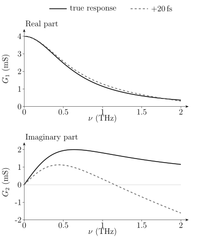
Calculated sheet response $G=G_0/(1-i\omega\tau)$ with $G_0=4\ \mathrm{mS}$, $\tau=0.25\ \mathrm{ps}$, and $n_s=3$. Solid curves show the true response; dashed curves show inversion with an uncorrected $+20\ \mathrm{fs}$ delay. Both give exactly the same transmitted field magnitude. Phase error alone reverses the inferred reactive sign at higher frequency. These curves are a teaching model, not measurements.

Keep a common absolute delay reference. Independently centering the two pulses removes real propagation delay unless the applied shifts are restored in the spectral phase. Phase unwrapping must also be checked against noise, the $2\pi$ branch, and the expected propagation time. Jepsen’s tutorial explains these distinct phase problems. Repeated insertion, fixed mounts, and independent thickness measurements help estimate the resulting uncertainty.

Atmospheric water has sharp rotational absorption throughout much of the THz band. Purge or vacuum, matched acquisition times, and inspection of known gas lines are standard controls. Numerical removal cannot recover information at a frequency where the sample signal has fallen below the noise floor.

Equilibrium versus driven response

Ordinary THz-TDS characterizes a stationary sample with a weak probe. In optical-pump–THz-probe spectroscopy, a pump changes the state and the measured quantity depends on pump–probe delay. Converting the differential field to a transient conductivity requires the excitation-depth profile, pump and probe penetration mismatch, nonstationarity during the THz waveform, and a multilayer nonequilibrium model.

Strong-field THz pulses can also drive nonlinear current, phonon, magnon, Josephson, or order-parameter dynamics. Once the response depends on field amplitude or waveform, a linear $\widetilde\sigma(\omega)$ is no longer a complete description.

What the measured features can tell you

Fit amplitude and phase together when both are measured. Interleave sample and reference scans to expose drift, and test whether the same model survives a change of thickness, polarization, temperature, or frequency range. Withayachumnankul and colleagues analyze uncertainty from the field measurements and sample parameters.

Observed feature	Possible interpretation	Useful distinguishing check
rolloff in $\sigma_1$ with dispersive $\sigma_2$	current relaxation	dc response and both complex components
increased transmission below a transition	changed absorption or reflection	recover the complex film response
$\sigma_2\propto1/\omega$ over a finite band	superconducting stiffness or a narrow normal Drude response	lower frequencies, missing area, and magnetic screening
absorption onset	an allowed excitation scale	matrix elements, disorder, excitons, and momentum assistance
a polar resonance	an electrically active mode	polarization, mode symmetry, and substrate comparison
high reflectance near phonon scales	a possible Reststrahlen interval	the fitted dielectric sign and surface geometry
a delayed pulse replica	an internal reflection	group delay, thickness, and echo amplitude
narrow gas lines	absorption along the atmospheric path	matched purge and reference conditions

The strongest interpretation explains several observations with compatible parameters. A causal fit to one spectrum is useful, but does not by itself identify a unique microscopic mechanism.

Exercises

1. Convert a terahertz scale

Convert $2.50\ \mathrm{THz}$ to meV, reciprocal centimetres, and vacuum wavelength.

Solution

Using the frequency conversions above,

$$\begin{aligned} E &= (2.50)(4.13567)\ \mathrm{meV} \\ &= 10.34\ \mathrm{meV}, \\[4pt] \widetilde\nu &= (2.50)(33.3564)\ \mathrm{cm}^{-1} \\ &= 83.39\ \mathrm{cm}^{-1}, \\[4pt] \lambda_0 &= \frac{299.792\ \mathrm{\mu m}}{2.50} \\ &= 119.9\ \mathrm{\mu m}. \end{aligned}$$

This lies in the overlap commonly called terahertz and far infrared.

2. Invert a thin-film transmission

A $100\ \mathrm{nm}$ film lies on a substrate with $n_s=3.0$. At one frequency the complex film-plus-substrate transmission relative to a matched bare substrate is

$$\widetilde t_{\mathrm{rel}} = 0.80-0.10i.$$

Use the thin-film expression to estimate sheet conductance and bulk conductivity, assuming that the bound-charge contribution is negligible at this frequency.

Solution

First,

$$\begin{aligned} \frac{1}{0.80-0.10i} &=\frac{0.80+0.10i}{0.65}\\ &=1.23077+0.15385i. \end{aligned}$$

Therefore

$$\begin{aligned} \widetilde G &= \frac{4}{376.73\ \Omega} \left( 0.23077+0.15385i \right) \\ &\simeq \left( 2.45+1.63i \right) \times10^{-3}\ \mathrm S. \end{aligned}$$

With $d=1.00\times10^{-7}\ \mathrm m$,

$$\widetilde\sigma = \frac{\widetilde G}{d} \simeq \left( 2.45+1.63i \right) \times10^4\ \mathrm{S\,m^{-1}}.$$

The result inherits the thin-film, matched-substrate, normal-incidence, and time-convention assumptions.

3. Read a Drude point

A one-component Drude response has $\sigma_0=4.00\times10^4\ \mathrm{S\,m^{-1}}$ and $\tau=0.250\ \mathrm{ps}$. Find $\sigma_1$, $\sigma_2$, and their ratio at $\nu=0.800\ \mathrm{THz}$.

Solution

The dimensionless frequency is

$$\begin{aligned} \omega\tau&=2\pi\nu\tau\\ &=2\pi(0.800)(0.250)\\ &\simeq1.257. \end{aligned}$$

Here $1\ \mathrm{THz}\times1\ \mathrm{ps}=1$. For

$$\widetilde\sigma = \frac{\sigma_0}{1-i\omega\tau},$$

one has

$$\begin{aligned} \sigma_1 &= \frac{\sigma_0}{1+(\omega\tau)^2} \simeq 1.55\times10^4\ \mathrm{S\,m^{-1}}, \\ \sigma_2 &= \frac{\sigma_0\omega\tau}{1+(\omega\tau)^2} \simeq 1.95\times10^4\ \mathrm{S\,m^{-1}}, \\ \frac{\sigma_2}{\sigma_1} &= \omega\tau \simeq 1.257. \end{aligned}$$

A measured ratio inconsistent with this value would reject the one-component parameter set even if one component alone looked plausible.

4. Infer a penetration depth

After subtracting regular dielectric and quasiparticle terms, a superconductor has $\sigma_2=3.00\times10^5\ \mathrm{S\,m^{-1}}$ at $\nu=0.500\ \mathrm{THz}$. Assuming $\sigma_2=D_s/\omega$, estimate $\lambda$.

Solution

The stiffness is

$$\begin{aligned} D_s &= \omega\sigma_2 \\ &= (3.14159\times10^{12}\ \mathrm{s^{-1}}) \times(3.00\times10^5\ \mathrm{S\,m^{-1}}) \\ &= 9.42\times10^{17} \ \mathrm{S\,m^{-1}\,s^{-1}}. \end{aligned}$$

Then

$$\begin{aligned} \lambda &= \frac{1}{\sqrt{\mu_0D_s}} \\ &\simeq 9.19\times10^{-7}\ \mathrm m \\ &= 0.919\ \mathrm{\mu m}. \end{aligned}$$

If regular terms were not removed, this procedure would misassign their reactive weight to the condensate.

5. Locate a polariton frequency

An ideal one-mode polar dielectric has the factorized response

$$\varepsilon(\nu) = 4\, \frac{3^2-\nu^2}{2^2-\nu^2},$$

where all frequencies are in THz, the TO pole is at $2\ \mathrm{THz}$, and the LO zero is at $3\ \mathrm{THz}$. Determine $\varepsilon(0)$, identify the negative-permittivity interval, and find the large-momentum vacuum-interface surface-polariton asymptote $\varepsilon=-1$. Does this frequency describe every momentum on the surface branch?

Solution

At zero frequency,

$$\varepsilon(0) = 4\,\frac{9}{4} = 9.$$

For $2<\nu<3\ \mathrm{THz}$, the denominator is negative while the numerator is positive, so $\varepsilon<0$. This is the ideal Reststrahlen interval.

At a vacuum interface,

$$4\frac{9-\nu^2}{4-\nu^2} = -1,$$

so

$$\begin{aligned} 36-4\nu^2&=-4+\nu^2,\\ \nu&=\sqrt{8}\ \mathrm{THz}\\ &\simeq2.83\ \mathrm{THz}. \end{aligned}$$

It lies between the $2\ \mathrm{THz}$ TO pole and $3\ \mathrm{THz}$ LO zero. The finite-momentum bound branch satisfies $q_\parallel=(\omega/c)\sqrt{\varepsilon/(\varepsilon+1)}$ and requires $\varepsilon<-1$. It approaches $2.83\ \mathrm{THz}$ only as $q_\parallel\to\infty$ in this lossless local model.

6. Echoes and resolution

A nondispersive substrate is $0.500\ \mathrm{mm}$ thick with $n_s=n_g=3.40$. Estimate its round-trip echo delay. Compare the Fourier-grid scales for a trace gated just before the echo and for an $80\ \mathrm{ps}$ trace in which echoes are modeled.

Solution

The echo delay is

$$\begin{aligned} \Delta t_{\mathrm{echo}} &= \frac{2n_sd_s}{c} \\ &= \frac{ 2(3.40)(0.500\times10^{-3}\ \mathrm m) }{ 2.998\times10^8\ \mathrm{m\,s^{-1}} } \\ &\simeq 11.3\ \mathrm{ps}. \end{aligned}$$

A pre-echo gate has a frequency scale no finer than roughly

$$\Delta\nu_{\mathrm{gate}} \sim \frac{1}{11.3\ \mathrm{ps}} \simeq 0.088\ \mathrm{THz}.$$

An $80\ \mathrm{ps}$ modeled trace has

$$\Delta\nu_{80} \sim \frac{1}{80\ \mathrm{ps}} = 0.0125\ \mathrm{THz}.$$

The longer trace can resolve narrower structure only if the echo model, timing stability, and dynamic range are trustworthy.

7. A phase error with unchanged transmitted power

At $1\ \mathrm{THz}$, a film on a substrate with $n_s=3$ has $G=(1.0+2.0i)\ \mathrm{mS}$. The sample waveform is accidentally delayed by $20\ \mathrm{fs}$ relative to its reference. Estimate the admittance error to first order and decide whether comparing field magnitudes reveals it.

Solution

The unwanted phase is

$$\begin{aligned} \phi&=\omega\delta t\\ &=2\pi(10^{12})(20\times10^{-15})\\ &\simeq0.126. \end{aligned}$$

With $C=4/Z_0\simeq10.62\ \mathrm{mS}$,

$$\begin{aligned} \delta G&\simeq-i\phi(C+G)\\ &\simeq(0.251-1.46i)\ \mathrm{mS}. \end{aligned}$$

The exact expression gives $G_{\mathrm{app}}\simeq(1.16+0.528i)\ \mathrm{mS}$. The first-order estimate is useful for scale and sign; its real component is noticeably affected by the second-order term. Since $|e^{i\omega\delta t}|=1$, neither the spectral field magnitude nor its squared magnitude detects this delay. A phase reference is essential.

References

• D. N. Basov, R. D. Averitt, D. van der Marel, M. Dressel, and K. Haule, “Electrodynamics of Correlated Electron Materials,” Reviews of Modern Physics 83, 471–541 (2011), doi:10.1103/RevModPhys.83.471.
• J. D. Caldwell et al., “Low-Loss, Infrared and Terahertz Nanophotonics Using Surface Phonon Polaritons,” Nanophotonics 4, 44–68 (2015), doi:10.1515/nanoph-2014-0003.
• R. A. Ferrell and R. E. Glover III, “Conductivity of Superconducting Films: A Sum Rule,” Physical Review 109, 1398–1399 (1958), doi:10.1103/PhysRev.109.1398.
• P. U. Jepsen, “Phase Retrieval in Terahertz Time-Domain Measurements: a “how to” Tutorial,” Journal of Infrared, Millimeter, and Terahertz Waves 40, 395–411 (2019), doi:10.1007/s10762-019-00578-0.
• M. Koch, D. M. Mittleman, J. Ornik, and E. Castro-Camus, “Terahertz Time-Domain Spectroscopy,” Nature Reviews Methods Primers 3, 48 (2023), doi:10.1038/s43586-023-00232-z.
• A. B. Kuzmenko, “Kramers–Kronig Constrained Variational Analysis of Optical Spectra,” Review of Scientific Instruments 76, 083108 (2005), doi:10.1063/1.1979470.
• R. H. Lyddane, R. G. Sachs, and E. Teller, “On the Polar Vibrations of Alkali Halides,” Physical Review 59, 673–676 (1941), doi:10.1103/PhysRev.59.673.
• D. C. Mattis and J. Bardeen, “Theory of the Anomalous Skin Effect in Normal and Superconducting Metals,” Physical Review 111, 412–417 (1958), doi:10.1103/PhysRev.111.412.
• M. Tinkham and R. A. Ferrell, “Determination of the Superconducting Skin Depth from the Energy Gap and Sum Rule,” Physical Review Letters 2, 331–333 (1959), doi:10.1103/PhysRevLett.2.331.
• W. Withayachumnankul, B. M. Fischer, H. Lin, and D. Abbott, “Uncertainty in Terahertz Time-Domain Spectroscopy Measurement,” Journal of the Optical Society of America B 25, 1059–1072 (2008), doi:10.1364/JOSAB.25.001059.
• W. Zimmermann, E. H. Brandt, M. Bauer, E. Seider, and L. Genzel, “Optical Conductivity of BCS Superconductors with Arbitrary Purity,” Physica C 183, 99–104 (1991), doi:10.1016/0921-4534(91)90771-P.

Further reading

• M. Dressel and G. Grüner, Electrodynamics of Solids: Optical Properties of Electrons in Matter (Cambridge University Press, 2002), doi:10.1017/CBO9780511606168. A systematic treatment of optical response, boundary conditions, and spectral-weight analysis.