Hall Measurements

A Hall measurement drives a longitudinal current and records a transverse voltage while an axial magnetic field, magnetization, or another time-reversal-odd variable is controlled. The raw voltage is not yet a Hall coefficient. It can contain thermoelectric offset, longitudinal pickup from contact misalignment, inductive voltage, contact asymmetry, field history, nonlinear response, and several parallel conduction channels.

The central task is to separate a transverse response from offsets, then decide what physical model can explain it. Record both current polarities and both field directions, together with the preparation of any magnetic state. A carrier density follows only after geometry, linear response, and the relevant carrier model have been checked.

Required background. Transport Measurements supplies terminal labeling, contact geometry and linear-response checks. Hall Effect supplies the signed transverse response and the assumptions behind carrier-density inference. Conventions for Quantum Matter fixes charge, field orientation and conductivity-tensor conventions.

Hall voltage and its sign

Fix a right-handed $(x,y,z)$ frame before connecting the voltmeter:

• conventional current $I>0$ flows along $+\hat{\mathbf x}$;
• magnetic induction $\mathbf B=B_z\hat{\mathbf z}$;
• the transverse voltage is $V_y=V_{\mathrm{bottom}}-V_{\mathrm{top}}$, with the top edge at larger $y$;
• the longitudinal voltage is $V_x=V_{\mathrm{upstream}}-V_{\mathrm{downstream}}$ under a declared lead order;
• $R_{yx}=V_y/I$ and $R_{xx}=V_x/I$ are terminal resistances;
• the magnetic field coordinate is $B$, not an unlabeled mixture of $B$ and applied $H$.

For labeled contacts, $V_{ab}=V_a-V_b$. Since $\mathbf E=-\nabla V$, a uniform transverse field gives $V_y=wE_y$. These conventions make the sign of a weak one-carrier Hall slope match the signed carrier charge: negative for electrons and positive for holes. Swapping the voltage leads changes the raw voltage sign. Reversing the physical current changes both the linear-response voltage and the signed current, so their ratio is unchanged. A sign error occurs if one polarity changes without updating its definition. Check the complete wiring and field direction, preferably with a known reference sample.

Hall-bar geometry

An ideal Hall bar has a long uniform channel, current contacts spanning the ends, narrow voltage arms, and paired transverse probes at the same longitudinal coordinate. The longitudinal pair samples the potential gradient along the bar; the transverse pair samples the cross-channel potential difference.

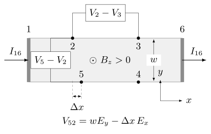
Current enters contact 1 and leaves contact 6. The longitudinal reading is $V_{23}=V_2-V_3$; the transverse reading is $V_{52}=V_5-V_2$. With uniform fields, the displacement shown gives $V_{52}=wE_y-\Delta x E_x$: the lower probe also samples the longitudinal voltage gradient. The ideal Hall pair has $\Delta x=0$. Voltage probes draw negligible current, and $B_z>0$ points out of the page.

For a homogeneous three-dimensional bar of thickness $t$ with uniform current density,

$$\rho_{yx} = t\,R_{yx}, \qquad \rho_{xx} = R_{xx}\frac{wt}{L}.$$

The Hall conversion does not contain the channel width because the wider current cross section and the longer transverse voltage path cancel in the ideal continuum geometry. That cancellation is not universal for finite voltage arms, invasive metal overlaps, irregular shapes, current jets, edge-dominated transport, or spatially varying conductivity.

For a two-dimensional conducting sheet, $R_{yx}$ is already the sheet Hall resistivity. Converting it to a three-dimensional $\rho_{yx}$ by multiplying by the physical thickness asserts that the current is uniformly distributed through that thickness. Surface states, parallel layers, accumulation regions, and partially depleted films violate that assertion.

Current contacts should spread current across the width before it reaches the voltage probes. Keep voltage arms narrow, measure their positions, and check for metal bridges, cracks, leakage, or nonlinear contacts. Invasive probes can shunt the Hall field rather than merely sample it (Gluschke et al., 2020). A uniform outline also does not guarantee a uniform carrier density; Bierwagen et al. (2008) discuss how inhomogeneity can even reverse the apparent carrier sign in van der Pauw measurements.

van der Pauw geometry

A uniform, isotropic, simply connected sheet with four sufficiently small contacts on its boundary supports both sheet-resistance and Hall measurements. Current is driven through one opposing contact pair and transverse voltage read across the other; current and field are reversed, and the diagonal configurations are exchanged.

The archived NIST procedure below gives an explicit acquisition sequence. Its redundant configurations test contact placement, sample uniformity, reversal consistency, and reciprocity. The method loses its guarantee when contacts lie in the interior, the sample contains a hole, thickness or carrier density varies appreciably, or anisotropy is ignored. Transport Measurements gives the sheet-resistance equation and its geometric assumptions.

From raw voltage to Hall resistance

A useful contamination model

A transverse record can be organized schematically as

$$V_y^{\mathrm{raw}} ={} V_{\mathrm{off}} + I R_{yx}(B,\mathcal H) + \epsilon I R_{xx}(B,\mathcal H) + V_{\mathrm{ind}}(\dot B) + V_{\mathrm{th}}.$$

$\epsilon$ parameterizes longitudinal pickup, often from contact misalignment or current distortion. $V_{\mathrm{off}}$ and $V_{\mathrm{th}}$ need not be field independent, while $V_{\mathrm{ind}}$ depends on sweep rate and loop area. It is a small-signal approximation: heating or changes in magnetic state can couple these contributions, so a single subtraction need not remove them.

Current reversal first

At fixed field and magnetic state, form the current-odd voltage

$$V_y^{I-}(B;\mathcal H) ={} \frac{1}{2} \bigl[ V_y(+I,B;\mathcal H) -V_y(-I,B;\mathcal H) \bigr].$$

This rejects static current-even offsets. It does not reject Joule-heating contributions that change resistance by an amount proportional to $I^2$ and therefore generate an odd $I^3$ voltage. Several excitation amplitudes are needed to establish a linear range.

Then separate field parity

Write $V^{s_I,s_B}=V_y(s_I I,s_B B)$ for states prepared by a matched protocol. The current-odd, field-odd Hall channel is

$$R_{yx}^{I-,B-}(B) ={} \frac{1}{4I} \bigl[ V^{+,+}-V^{-,+} -V^{+,-}+V^{-,-} \bigr].$$

The corresponding current-odd, field-even diagnostic is

$$R_{yx}^{I-,B+}(B) ={} \frac{1}{4I} \bigl[ V^{+,+}-V^{-,+} +V^{+,-}-V^{-,-} \bigr].$$

For a reversible nonmagnetic sample, longitudinal pickup is commonly field even and appears in $R_{yx}^{I-,B+}$, while the ordinary Hall signal appears in $R_{yx}^{I-,B-}$. The decomposition itself is exact for the four numbers. Interpreting the odd channel as Hall response requires matched sample states and controlled geometry. A field-even transverse voltage can also be physical, for example from in-plane anisotropy; it is not automatically a wiring error. In a mesoscopic four-terminal device, even a nominal longitudinal transfer resistance need not be even in field. Lead reciprocity is the more general constraint (Büttiker, 1986).

Reciprocity and lead exchange

Let $R_{ab,cd}=(V_c-V_d)/I_{ab}$, where positive current enters $a$ and leaves $b$. For a fixed sample in linear response, microscopic reversibility gives

$$R_{ab,cd}(B,\mathcal M) =R_{cd,ab}(-B,-\mathcal M).$$

Here $\mathcal M$ stands for every internal time-reversal-odd order parameter, not just the net magnetization. This compares exchanged current and voltage pairs, with the field and magnetic order reversed. It does not require $R_{ab,cd}(B)=R_{ab,cd}(-B)$. Casimir (1945) gives the general principle; Büttiker (1986) applies it to coherent multiterminal conductors.

Plan lead exchange into the same measurement sequence. A mismatch first calls for checks of excitation, contact stability, temperature drift, and magnetic preparation before concluding that the assumed response regime fails.

Carrier density, sign, and mobility

One-carrier sheet inference

Define the low-field sheet Hall slope

$$S_{\mathrm H}^{2\mathrm D} \equiv \left. \frac{dR_{yx}^{I-,B-}}{dB} \right|_{B\to0}.$$

For one isotropic carrier type with Hall factor unity,

$$n_s = \frac{1}{e\lvert S_{\mathrm H}^{2\mathrm D}\rvert}, \qquad \operatorname{sgn}(q) = \operatorname{sgn}(S_{\mathrm H}^{2\mathrm D}).$$

Here $e>0$ and $n_s$ is a positive sheet density. A conducting thickness $t$ gives $n=n_s/t$ only if the current-carrying layer is known and uniform.

If the same channel also produces sheet resistance $R_{\square}$, the one-carrier Hall mobility is

$$\mu_{\mathrm H} = \frac{ \lvert S_{\mathrm H}^{2\mathrm D}\rvert }{R_{\square}} = \frac{1}{e n_s R_{\square}}.$$

This is a model-derived mobility, not a directly recorded velocity. Parallel channels, anisotropic scattering, magnetic response, or an energy-dependent relaxation time break the simple identification.

Hall factor

In semiconductor transport, a Hall factor $r_{\mathrm H}$ is often introduced so that the measured slope is $r_{\mathrm H}/(n_s q)$. Then the apparent Hall density is $n_s/r_{\mathrm H}$ and $\mu_{\mathrm H}=r_{\mathrm H}\mu_{\mathrm{drift}}$. The factor depends on band structure, scattering, degeneracy, and temperature. Setting it to one should be stated as an approximation.

A sign assignment needs a slope resolved from zero and calibrated field, current, and voltage polarities. Even then, a positive weak-field slope can coexist with electron pockets if higher-mobility holes dominate the transverse response. It does not identify the charge of every mobile excitation.

Ordinary, anomalous, and quantum Hall signals

Ordinary Hall response

An ordinary one-carrier response is odd in field and, in the simplest model, linear. Check consistency across excitation amplitudes and lead configurations, then use longitudinal transport and another density-sensitive measurement to test that interpretation. A straight Hall trace alone is insufficient: a multiband conductor can look linear over a narrow field window, and an anomalous contribution can look linear before magnetization saturates. Hall factors and parallel conduction can change the inferred density even when the trace is straight.

Anomalous Hall response

In a magnetic conductor, analysts often write the measured Hall resistivity as an ordinary background plus an anomalous term. Treat this as a model decomposition. Subtracting a high-field line assumes that the ordinary coefficient is field independent and that the anomalous response has reached a known high-field behavior.

Measure longitudinal and transverse response together on both sweep branches, and compare with magnetization or another probe of magnetic order under the same preparation. Temperature, angle, thickness, and disorder dependence help distinguish mechanisms; Nagaosa et al. (2010) review their physical origins. If the Hall angle is appreciable, invert the full tensor rather than using a small-angle approximation.

An anomalous Hall loop need not be proportional to net magnetization. Berry curvature, skew scattering, side jump, noncollinear order, and multiple magnetic regions can contribute. Hall Effect develops those mechanisms.

Quantum Hall response

A quantum Hall claim is based on a correlated longitudinal and transverse pattern, not a flat-looking segment:

• $\lvert R_{yx}\rvert$ approaches $h/(\nu e^2)$ for an identified positive integer or fractional filling magnitude $\nu$;
• $R_{xx}$ develops a corresponding minimum and ideally becomes unresolved;
• the feature persists over a field or density interval;
• current is below the breakdown threshold;
• contact and lead mixing are tested;
• temperature and device-size dependence are consistent with the proposed gap and edge transport.

A useful magnitude residual is

$$\delta_\nu \equiv \frac{\lvert R_{yx}\rvert}{h/(\nu e^2)} -1.$$

The sign of $R_{yx}$ is recorded separately under the terminal and field convention above; using a magnitude for this residual does not discard that sign from the data. A small $\delta_\nu$ with appreciable $R_{xx}$ is not yet a metrological plateau. The finite longitudinal signal can mix into $R_{yx}$ and indicates dissipation or incomplete quantization. Integer Quantum Hall Effect explains plateau formation and edge transport, starting from the measurements of von Klitzing, Dorda, and Pepper (1980).

Multiband and parallel conduction

Coexisting bulk carrier types add conductivity tensors before inversion. Distinct layers instead add sheet conductance tensors, provided they share the same in-plane electric field and their contacts equilibrate the layers:

$$\mathbf G_{\mathrm{tot}}=\sum_a t_a\boldsymbol\sigma^{(a)}, \qquad \boldsymbol\rho^{\square}=\mathbf G_{\mathrm{tot}}^{-1}.$$

Each $t_a\boldsymbol\sigma^{(a)}$ has units of siemens; a genuinely two-dimensional channel contributes its sheet tensor directly. Do not add a bulk conductivity in $\mathrm{S\,m^{-1}}$ to a sheet conductance in $\mathrm S$. A channel confined to an edge, or layers with poorly equilibrated contacts, need a terminal-transport model rather than this local uniform-field sum. See Landauer–Büttiker Formalism for the contact-based description.

For an isotropic sheet with antisymmetric Hall part, inversion gives

$$G_{xx}=\frac{\rho_{xx}^{\square}} {(\rho_{xx}^{\square})^2+(\rho_{yx}^{\square})^2}, \qquad G_{yx}=\frac{-\rho_{yx}^{\square}} {(\rho_{xx}^{\square})^2+(\rho_{yx}^{\square})^2}.$$

Convert the longitudinal terminal resistance first: $\rho_{xx}^{\square}=R_{xx}w/L$, while $\rho_{yx}^{\square}=R_{yx}$ in an ideal Hall bar. Taking the reciprocal of each measured resistance separately misses both geometry and tensor mixing. An anisotropic sheet requires its complete tensor.

The familiar two-carrier model contains four positive parameters, $n,p,\mu_e,\mu_h$, before offsets, geometry uncertainty, or field dependence are added. A short weak-field Hall trace generally cannot determine all four independently. A wide field range can contain more information, but parameter count alone does not establish whether a fit is identifiable. At minimum:

1. fit $\rho_{xx}(B)$ and $\rho_{yx}(B)$ simultaneously in tensor form;
2. report parameter covariance and sensitivity to the field window;
3. repeat across temperature or gate voltage with physically justified shared parameters;
4. constrain density or Fermi-surface area with capacitance, stoichiometry, spectroscopy, or quantum oscillations;
5. test whether an additional parallel channel changes the conclusion.

Adding a third carrier because residuals remain does not automatically improve physical inference. It may only make a flexible inverse problem less identifiable.

Hysteresis and magnetic effects

History is an experimental coordinate

In a magnetic sample, write $R_{yx}(B;\mathcal H)$, where $\mathcal H$ specifies sweep direction, saturation or cooling preparation, maximum field, wait time, and any gate or current pulse that may change domains. Field alone does not specify the state.

For a symmetric major hysteresis loop, an upsweep prepared at negative saturation and a downsweep prepared at positive saturation can satisfy

$$\mathcal M_{\uparrow}(B)=-\mathcal M_{\downarrow}(-B).$$

These opposite-branch points are then the appropriate time-reversed pair; remaining on one branch is not inherently safer. Exchange bias, incomplete saturation, training, relaxation, or different domain patterns can destroy this relation. Preserve both branches and test their magnetic preparation before pairing points. Even equal and opposite net magnetizations need not establish that the full internal configurations are time reverses.

Longitudinal and planar Hall mixing

Anisotropic magnetoresistance can generate a planar Hall voltage when magnetization lies in the plane. Its field parity and angular dependence differ from an axial ordinary Hall signal, but domain reversal and misalignment can mix channels. A three-axis angle study should report the actual field vector and mechanical zero, not only the rotator readout.

Residual humps are not direct topology measurements

A common procedure fits an ordinary background, subtracts an anomalous term proportional to magnetization, and labels the remaining hump “topological Hall.” The residual inherits every error in both backgrounds. Multiple magnetic regions with different coercivities and opposite anomalous-Hall signs can create a similar feature without a skyrmion phase (Gerber, 2018).

A real-space-topology claim needs orthogonal evidence such as imaging or scattering, a texture model, field-angle and thickness systematics, and agreement among magnetization, transport, and phase boundaries. Skyrmions and Magnetic Textures explains how magnetic texture produces an emergent field and what additional observations test that interpretation.

Uncertainty and detection limits

For a one-carrier sheet density $n_s=1/(e|S_{\mathrm H}^{2\mathrm D}|)$, the relative standard uncertainty is approximately

$$\frac{u(n_s)}{n_s} \simeq \frac{ u(S_{\mathrm H}^{2\mathrm D}) }{ \lvert S_{\mathrm H}^{2\mathrm D}\rvert },$$

when the slope uncertainty is small compared with its magnitude and the one-carrier model is valid. The charge $e$ is exact in the SI. The slope uncertainty must include voltage noise, current calibration, field calibration, drift, field-window choice, and correlated residuals. For bulk density $n=n_s/t$, thickness uncertainty and uncertainty in the electrically active layer must be added.

When a symmetric two-field estimate is appropriate,

$$S_{\mathrm H}^{2\mathrm D} \simeq \frac{ V_y^{I-}(+B)-V_y^{I-}(-B) }{ 2IB }.$$

This estimator assumes linearity between the two fields. A regression over many points should report the model, weighting, covariance, and sensitivity to the fit interval. If a plausible slope interval crosses zero, neither a carrier sign nor a finite upper density bound follows from this inverse formula. The uncertainty of $1/|S_{\mathrm H}^{2\mathrm D}|$ is then strongly asymmetric; a symmetric error bar obtained by linear propagation is misleading. Model uncertainty from additional channels is separate from voltage noise.

For $\mu_{\mathrm H}=|S_{\mathrm H}^{2\mathrm D}|/R_{\square}$, slope and sheet-resistance uncertainties can be correlated because the same contacts, geometry, temperature, and conduction channels enter both. Propagating them as independent can misstate the mobility uncertainty. The covariance treatment in JCGM 100:2008 applies; a fit should also show its field interval and residuals so the reader can assess the assumed linear law.

Exercises

1. Signed sheet density

With the bottom-minus-top voltage convention of this page, a device carrying $I=10.0\,\mu\mathrm A$ at $B=+1.00\,\mathrm T$ has current-odd transverse voltage $V_y^{I-}=-2.00\,\mathrm{mV}$ after field-even pickup is removed. Assume one-carrier linear response. Find the sheet Hall slope, carrier sign, and sheet density.

Solution

The Hall resistance at this field is

$$R_{yx} = \frac{-2.00\,\mathrm{mV}} {10.0\,\mu\mathrm A} = -200\,\Omega.$$

Linearity through the origin gives $S_{\mathrm H}^{2\mathrm D}=-200\,\Omega\,\mathrm T^{-1}$. The negative sign identifies electrons under the declared convention. The sheet density is

$$\begin{aligned} n_s &= \frac{1}{ e\lvert S_{\mathrm H}^{2\mathrm D}\rvert } \\ &= 3.12\times10^{16}\,\mathrm m^{-2} \\ &= 3.12\times10^{12}\,\mathrm{cm}^{-2}. \end{aligned}$$

The result is model conditional: it assumes one carrier type and Hall factor unity.

2. Four-state extraction

At one field magnitude and $I=100\,\mu\mathrm A$, the transverse voltages in microvolts are

$$\begin{aligned} V^{+,+}&=310, & V^{-,+}&=-250, \\ V^{+,-}&=150, & V^{-,-}&=-90. \end{aligned}$$

Find the current-odd response at each field, then the field-odd and field-even transfer resistances.

Solution

At positive and negative field,

$$\begin{aligned} V_y^{I-}(+B) &= \frac{310-(-250)}{2}\,\mu\mathrm V \\ &= 280\,\mu\mathrm V, \\ V_y^{I-}(-B) &= \frac{150-(-90)}{2}\,\mu\mathrm V \\ &= 120\,\mu\mathrm V. \end{aligned}$$

The odd and even voltages are therefore $80\,\mu\mathrm V$ and $200\,\mu\mathrm V$. Dividing by current gives

$$R_{yx}^{I-,B-} = 0.80\,\Omega, \qquad R_{yx}^{I-,B+} = 2.00\,\Omega.$$

The larger field-even channel is consistent with substantial longitudinal pickup. It should be reported and investigated, not silently discarded.

3. A Hall slope close to zero

Under a one-carrier model, an estimate gives $S=-2.0\,\Omega\,\mathrm T^{-1}$ with standard uncertainty $u(S)=1.5\,\Omega\,\mathrm T^{-1}$. Treat $[-5,1]\,\Omega\,\mathrm T^{-1}$ as an approximate coverage interval. What goes wrong with quoting only the central Hall density and a symmetric uncertainty? How does an unknown conducting thickness affect the conclusion?

Solution

The central estimate is $n_{\mathrm H}=1/(e|S|)=3.12\times10^{18}\,\mathrm m^{-2}$. Linear propagation would give a 75% relative uncertainty, already too large to justify linearizing the reciprocal. The stated interval includes positive and negative slopes and arbitrarily small nonzero magnitudes. It therefore leaves the carrier sign unresolved and maps to unbounded density above; its largest slope magnitude gives a conditional lower bound $1/(5e)=1.25\times10^{18}\,\mathrm m^{-2}$. Exactly zero slope has no finite-density realization in this ideal single-carrier formula.

If the one-carrier model is wrong, even that bound need not apply: cancellation between electron and hole contributions can give zero Hall slope at finite density. A thickness uncertainty enters only the conversion $n=n_s/t$ after a reliable sheet density exists. It cannot rescue an unresolved Hall slope.

4. A positive slope with more electrons

In the weak-field two-carrier model, the Hall numerator is proportional to $p\mu_h^2-n\mu_e^2$. Consider $n=4$ and $p=2$ in common density units, with $\mu_e=1000$ and $\mu_h=2000$ in common mobility units. Determine the Hall sign and explain the lesson.

Solution

The two weighted terms are

$$p\mu_h^2 = 2(2000)^2 = 8.0\times10^6,$$

and

$$n\mu_e^2 = 4(1000)^2 = 4.0\times10^6.$$

The numerator is positive, so the weak-field Hall slope is hole-like even though electrons are twice as numerous. Hall sign is mobility weighted in a multiband conductor; it is not a census of every carrier or Fermi-surface pocket.

5. Which hysteresis branches should be paired?

A toy symmetric magnetic loop has

$$\begin{aligned} m_{\uparrow}(B)&=\tanh[(B-B_c)/b],\\ m_{\downarrow}(B)&=\tanh[(B+B_c)/b], \end{aligned}$$

where $m=M/M_s$, $B_c>0$, and $b>0$ sets the switching width. Suppose $R_{yx}=S_0B+A m$. Which branch at $-B$ is the time reverse of an upsweep point at $+B$? Does the half-difference isolate the ordinary term $S_0B$? What changes if both loops are shifted by the same exchange-bias field $B_E$?

Solution

Oddness of $\tanh$ gives $m_{\downarrow}(-B)=-m_{\uparrow}(B)$. Thus

$$\frac{R_{\uparrow}(B)-R_{\downarrow}(-B)}2 =S_0B+A m_{\uparrow}(B).$$

Opposite branches form the correct pair in this model. Antisymmetrization retains the anomalous term as well as the ordinary one; it cannot separate them by parity. Same-branch pairing generally does not compare reversed magnetizations, particularly near switching.

With exchange bias, replace $B$ by $B-B_E$ in both magnetic curves. At fixed $B_E\ne0$, $m_{\downarrow}(-B)$ is no longer $-m_{\uparrow}(B)$. Reversing the pinning order, represented here by $B_E\to-B_E$, restores the relation. Real samples can have additional domain-state and relaxation differences beyond this one-variable model.

6. Is this a quantum Hall plateau?

Near a proposed filling-magnitude $\nu=2$ plateau, a device gives $\lvert R_{yx}\rvert=12.910\,\mathrm{k}\Omega$ and $R_{xx}=20\,\Omega$. Use $h/e^2=25\,812.807\,\Omega$ to calculate the magnitude residual $\delta_2$. Does the measurement establish a metrological plateau?

Solution

The ideal value is

$$\frac{h}{2e^2} = 12\,906.404\,\Omega.$$

Therefore

$$\begin{aligned} \delta_2 &= \frac{12\,910}{12\,906.404}-1 \\ &= 2.79\times10^{-4}. \end{aligned}$$

The Hall value is close at the $10^{-4}$ level, but $R_{xx}=20\,\Omega$ is clearly nonzero and can mix into the transverse channel. The observation is consistent with an emerging plateau, not by itself with metrological quantization. Current dependence, contact configuration, temperature, field width, and uncertainty must also be checked.

References

• O. Bierwagen, T. Ive, C. G. Van de Walle, and J. S. Speck, “Causes of Incorrect Carrier-Type Identification in van der Pauw–Hall Measurements”, Applied Physics Letters 93, 242108 (2008).
• M. Büttiker, “Four-Terminal Phase-Coherent Conductance”, Physical Review Letters 57, 1761–1764 (1986).
• H. B. G. Casimir, “On Onsager’s Principle of Microscopic Reversibility”, Reviews of Modern Physics 17, 343–350 (1945).
• A. Gerber, “Interpretation of Experimental Evidence of the Topological Hall Effect”, Physical Review B 98, 214440 (2018).
• J. G. Gluschke, J. Seidl, H. H. Tan, C. Jagadish, P. Caroff, and A. P. Micolich, “Impact of Invasive Metal Probes on Hall Measurements in Semiconductor Nanostructures”, Nanoscale 12, 20317–20325 (2020).
• Joint Committee for Guides in Metrology, Evaluation of Measurement Data—Guide to the Expression of Uncertainty in Measurement, JCGM 100:2008.
• N. Nagaosa, J. Sinova, S. Onoda, A. H. MacDonald, and N. P. Ong, “Anomalous Hall Effect”, Reviews of Modern Physics 82, 1539–1592 (2010).
• National Institute of Standards and Technology, “Resistivity and Hall Measurements”, archived measurement procedure and consistency checks.
• L. J. van der Pauw, “A Method of Measuring Specific Resistivity and Hall Effect of Discs of Arbitrary Shape,” Philips Research Reports 13, 1–9 (1958).
• K. von Klitzing, G. Dorda, and M. Pepper, “New Method for High-Accuracy Determination of the Fine-Structure Constant Based on Quantized Hall Resistance”, Physical Review Letters 45, 494–497 (1980).