Integer Quantum Hall Effect

The integer quantum Hall effect is the quantization of transverse electrical response in an effectively two-dimensional electronic system whose bulk is insulating at the Fermi level while chiral boundary channels remain conducting. In a Hall bar at low temperature and strong perpendicular magnetic field, the Hall resistance develops broad plateaus while the longitudinal resistance becomes very small:

$$\left|R_{yx}\right| = \frac{h}{N e^2}, \qquad R_{xx}\simeq0, \qquad N\in\mathbb N.$$

The striking feature is not merely that an ideal Landau-level model produces an integer. It is that a disordered, finite device with contacts can reproduce the same resistance over a finite interval of magnetic field or carrier density. Landau quantization supplies the levels, topology fixes the transverse response, localized bulk states widen the plateaus, and chiral edge channels connect that bulk response to a multiprobe measurement.

Here $N$ is the positive integer labeling a resolved electron Hall plateau. It is distinct from the continuously variable filling factor $\nu=n_{2\mathrm D}h/(eB)$. The distinction is essential for explaining a plateau: density can change while the Hall integer remains fixed.

Required background. Landau Levels supplies the spectrum, Degeneracy of Landau Levels supplies flux counting, and Hall Effect supplies the Hall-tensor and transport definitions.

Helpful background. Topology in Quantum Matter explains phase stability, while Chern Numbers and Chern Numbers in Band Theory supply the geometric and band-projector formulations, and Kubo Formula supplies the general response derivation.

Landau filling and quantized Hall response

Take a right-handed $(x,y,z)$ frame, a two-dimensional sample in the $xy$ plane, and

$$\mathbf B=B\hat{\mathbf z}, \qquad B>0.$$

The mobile particles are electrons of charge $q=-e$, where $e>0$. As on the Hall Effect page, write

$$\begin{pmatrix} j_x\\ j_y \end{pmatrix} = \begin{pmatrix} \sigma_{xx} & \sigma_{xy}\\ -\sigma_{xy} & \sigma_{xx} \end{pmatrix} \begin{pmatrix} E_x\\ E_y \end{pmatrix}.$$

The inverse tensor gives

$$\rho_{xx} = \frac{\sigma_{xx}} {\sigma_{xx}^2+\sigma_{xy}^2}, \qquad \rho_{yx} = \frac{\sigma_{xy}} {\sigma_{xx}^2+\sigma_{xy}^2}.$$

These tensor formulas assume a homogeneous isotropic two-dimensional bulk. Its $\rho_{yx}$ has units of resistance and can equal a measured Hall resistance in an ideal Hall-bar geometry with declared lead polarity. For anisotropy, invert the actual tensor; for a nonlocal edge device, solve the contact-current equations. A measured resistance is not automatically a local resistivity component. On a plateau, $\sigma_{xx}\to0$ gives

$$\rho_{yx}=\frac{1}{\sigma_{xy}}, \qquad \rho_{xx}\to0.$$

For the ordinary continuum electron Landau-level sequence at $B>0$, $\sigma_{xy}<0$. A general lattice Chern band can have either Hall sign; carrier charge and external field alone do not determine its Chern number. To keep the universal magnitudes visible while avoiding silent sign changes between common tensor conventions, this page writes

$$\left|\sigma_{xy}\right| = N\frac{e^2}{h}, \qquad \left|\rho_{yx}\right| = \frac{h}{N e^2}.$$

Signed formulas are stated explicitly when needed. Reversing $B$, reversing the carrier charge, reversing the orientation of the sample, or exchanging the tensor-index convention reverses the Hall sign but not the quantized magnitude.

Experimental Signature

The original observation used a silicon metal–oxide–semiconductor field-effect transistor, where a gate confines electrons to an inversion layer. Modern platforms include GaAs/AlGaAs heterostructures, graphene, oxide interfaces, and other effectively two-dimensional conductors. Material details change the accessible temperatures, fields, degeneracies, and plateau sequence, but the diagnostic logic is the same.

A four-terminal measurement separates the imposed current path from voltage probes that ideally draw no current. The original experiment was reported by von Klitzing, Dorda and Pepper (1980). As magnetic field or carrier density is swept:

1. $R_{yx}$ becomes nearly constant on a plateau;
2. $R_{xx}$ develops a deep minimum in the same interval;
3. transitions between adjacent plateaus coincide with peaks in $R_{xx}$;
4. the plateau value approaches $R_K/N$, where $R_K=h/e^2$;
5. the result is independent of the macroscopic aspect ratio after the Hall-bar geometry and lead configuration are treated correctly.

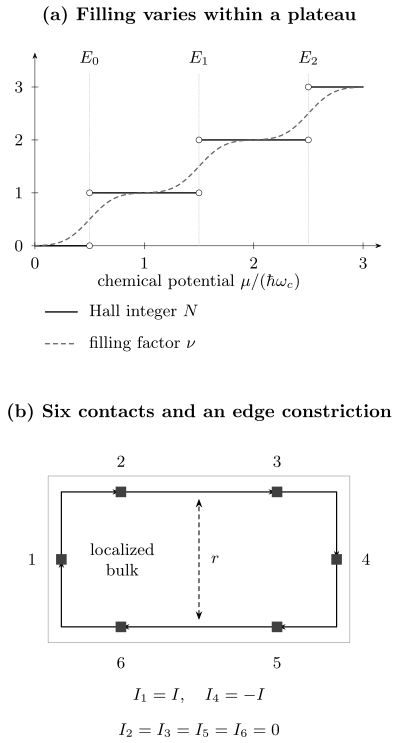
Above: a schematic localized-state model separates the smooth filling factor $\nu$ from the integer Hall label $N$. Each broadened level has a Gaussian density of states; the Hall integer changes only at the marked critical energy. This is an illustration of state counting, not a calculation of localization. Below: six ideal contacts absorb and repopulate the incoming edge channels. A constriction can mix opposite edges, parameterized by the total reflected channel weight $r$. The contact equations below determine the measured voltages; arrows specify channel propagation, not the sign of electron charge.

A low value of $R_{xx}$ alone is not enough. A short circuit, a superconducting path, contact failure, or an incorrectly symmetrized trace can also produce a small longitudinal voltage. Reliable identification requires the correlated Hall plateau, field-reversal checks, current-reversal checks, stable contacts, and a regime below quantum Hall breakdown.

Landau levels, filling and the plateau integer

For one resolved spin/valley component, each Landau level has one orbital state per flux quantum $\Phi_e=h/e$. In area $A$,

$$\begin{aligned} N_\Phi&=\frac{BA}{\Phi_e},\\ n_\Phi&=\frac{eB}{h}=\frac{1}{2\pi\ell_B^2},\\ \ell_B&=\sqrt{\frac{\hbar}{eB}}. \end{aligned}$$

Thus the filling factor is

$$\nu=\frac{N_{\rm e}}{N_\Phi} =\frac{n_{2\mathrm D}h}{eB}.$$

It counts particles per flux quantum and is generally not an integer. In the clean spin-resolved parabolic-band model,

$$E_n=\hbar\omega_c(n+1/2),\qquad \omega_c=\frac{eB}{m},$$

so filling exactly $N$ levels gives $\nu=N$. Spin splitting, valley splitting, disorder and interactions determine which levels are resolved. For example, the usual fourfold-degenerate graphene sequence has $|\sigma_{xy}|/(e^2/h) =2,6,10,\ldots$ away from neutrality, before degeneracy lifting. It is still integer charge Hall quantization, despite the offset from the parabolic-band sequence; see Graphene and Dirac Materials.

At fixed density, exact clean integer filling occurs only at $B_N=n_{2\mathrm D}h/(eN)$. Substituting this into the classical result $|\rho_{yx}|=B/(en_{2\mathrm D})$ reproduces $h/(Ne^2)$ at that field. This counting check does not explain a finite interval of constant resistance. Localized states allow $\nu$ to change while $N$ stays fixed.

For the illustrative figure, three Gaussian-broadened resolved levels have centers $E_j=j+1/2$, $j=0,1,2$, and width $\Gamma=0.18$ in cyclotron-energy units. With $F$ the unit-normal cumulative distribution,

$$\begin{aligned} \nu(\mu)&=\sum_{j=0}^2F\!\left(\frac{\mu-E_j}{\Gamma}\right),\\ N(\mu)&=\sum_{j=0}^2\Theta(\mu-E_j). \end{aligned}$$

The second line idealizes each critical energy as a zero-width transition. Between these energies, localized states change the first line without changing the second. At a critical energy the ideal plateau limit fails; the value assigned to the step function at its jump is not a Hall plateau.

Chiral Edge States

A confining potential turns the macroscopically degenerate bulk levels into dispersing states near a boundary. In Landau gauge, a momentum label fixes a guiding-center coordinate $Y$. If the confining potential $U(Y)$ varies slowly on the magnetic-length scale, the edge dispersion is approximately

$$E_n(k) \simeq \hbar\omega_c \left( n+\frac12 \right) + U(Y_k).$$

The group velocity is

$$v_n(k) = \frac{1}{\hbar} \frac{dE_n}{dk} \simeq \frac{1}{\hbar} \frac{dU}{dY} \frac{dY_k}{dk}.$$

The confining potential has opposite slope on opposite sides of a Hall bar. Thus the modes propagate in opposite coordinate directions on opposite edges, yet together circulate with one chirality around the sample boundary. At a given edge there is no nearby mode moving backward at the same energy in the ideal integer regime.

A reservoir sets the occupation of channels leaving it. In linear response, write $V_i$ for its electrochemical voltage and $I_i$ for the current injected into the device. For $N$ ideal channels following the arrows in the figure, the Landauer–Büttiker equations are

$$I_i=\frac{Ne^2}{h}(V_i-V_{i-1}),$$

with indices cyclic. Contact 1 supplies $I$, contact 4 receives it, and the other four contacts are voltage probes with $I_i=0$. Each voltage probe therefore takes the potential of its upstream reservoir:

$$V_2=V_3=V_1,\qquad V_5=V_6=V_4.$$

Choosing $V_4=0$ gives $I=(Ne^2/h)V_1$ and

$$\begin{aligned} R_{14,26}&\equiv\frac{V_2-V_6}{I}=\frac{h}{Ne^2},\\ R_{14,23}&\equiv\frac{V_2-V_3}{I}=0. \end{aligned}$$

The positive first ratio follows the specified contact order. Mapping it to the signed $\rho_{yx}$ above requires identifying the physical $x,y$ axes and voltage polarity. This avoids silently changing the Hall sign when a diagram is reflected. General channel transmission and reservoir conventions are developed in Landauer–Büttiker Formalism.

Chirality suppresses elastic backscattering on an isolated ideal edge because there is no outgoing backward channel there. Co-propagating channels can scatter into each other without generating longitudinal resistance when all are equally populated. Counterpropagating reconstructed branches, opposite-edge coupling and selective contacts require a fuller transmission calculation (Büttiker, 1988). Topology fixes a net chirality, not every microscopic branch.

A constriction separates two experimental checks

Let a constriction between contacts 2 and 3 mix the upper incoming channels from 2 with the lower incoming channels from 5. Let $r$ be the sum of reflection probabilities, with $0\leq r<N$. Ideal downstream probes then read

$$\begin{aligned} V_3&=\frac{(N-r)V_2+rV_5}{N},\\ V_6&=\frac{rV_2+(N-r)V_5}{N}. \end{aligned}$$

Since $V_2=V_1$ and $V_5=V_4=0$, $I=(N-r)(e^2/h)V_1$. Consequently,

$$\begin{aligned} R_{14,26}&=\frac{R_K}{N},\\ R_{14,23}&=\frac{r}{N(N-r)}R_K. \end{aligned}$$

The transverse ratio remains quantized in this ideal geometry even though the longitudinal resistance is nonzero. Thus a near-quantized Hall ratio alone does not establish a dissipationless metrological regime. For $N=2$ and $r=0.30$, the two ratios are $0.5R_K$ and $0.0882353R_K$. Other contact or scattering arrangements need not preserve the transverse ratio; the result here follows from the stated six-contact problem.

Bulk and edge are complementary

The bulk and edge descriptions answer different parts of the same experiment:

• the bulk Chern number fixes the net number and chirality of boundary modes relative to the exterior;
• localized bulk states allow the chemical potential to move without changing the Hall integer;
• edge-channel occupations determine terminal currents in the ideal contact model;
• contacts populate and equilibrate the incoming channels.

It is therefore misleading to ask whether the Hall current is “really” a bulk current or “really” an edge current without specifying geometry, equilibrium subtraction, and the measured observable. The topological response can be computed with periodic boundaries and no physical edge, while a Hall-bar voltage measurement necessarily involves boundaries and reservoirs.

Laughlin Flux-Insertion Argument

Place the two-dimensional system on a cylinder and thread magnetic flux $\Phi$ through its axis. Increasing the flux by one electronic flux quantum,

$$\Delta\Phi = \Phi_e = \frac{h}{e},$$

returns the Hamiltonian to a gauge-equivalent form. During the insertion, Faraday induction creates an electric field around the cylinder and transports charge from one boundary to the other.

With the bulk adiabatic/localization conditions maintained and an edge occupation protocol that follows the spectral transfer, one flux quantum produces integer charge flow. Fully adiabatic following of one unique finite-cylinder state across tiny opposite-edge avoided crossings is a different limit; the bulk gap alone does not specify the boundary occupations. Suppose the net transported charge magnitude is

$$\left|\Delta Q\right| = N e.$$

The integrated Hall response also gives

$$\left|\Delta Q\right| = \left|\sigma_{xy}\right| \Delta\Phi.$$

Therefore

$$\left|\sigma_{xy}\right| \frac{h}{e} = N e,$$

and hence

$$\left|\sigma_{xy}\right| = N\frac{e^2}{h}.$$

The argument isolates the two ingredients behind exact quantization: gauge equivalence after one flux quantum and integer charge spectral flow in a phase that does not become dissipative during the cycle. It does not by itself calculate every plateau sequence or describe localization quantitatively. Those require the microscopic spectrum, internal degeneracies, disorder, and contacts.

Chern Number Interpretation

For clean noninteracting electrons in a periodic two-dimensional system, use the oriented measure $dk_x\wedge dk_y$, the Berry connection $\mathcal A_n=i\langle u_n|\boldsymbol\nabla_{\mathbf k}u_n\rangle$, and $\Omega_n=\partial_{k_x}\mathcal A_{n,y}-\partial_{k_y}\mathcal A_{n,x}$. With the electron and conductivity-tensor conventions above, the Kubo formula can then be reorganized into the Thouless–Kohmoto–Nightingale–den Nijs expression

$$\sigma_{xy} = -\frac{e^2}{h}C_{\mathrm{occ}},$$

where

$$C_{\mathrm{occ}} = \frac{1}{2\pi} \sum_{n\in\mathrm{occ}} \int_{\mathrm{BZ}} \Omega_n(\mathbf k)\,d^2k.$$

The sign of $C_{\mathrm{occ}}$ follows the chosen Brillouin-zone orientation and Berry-curvature convention. With the complete convention block used here, the Chern and Hall signs are opposite: filled continuum electron Landau levels at $B>0$ have $C_{\mathrm{occ}}>0$ and $\sigma_{xy}<0$. Each resolved filled Landau level changes the magnitude of the Hall integer by one. A source using $\mathcal A=-i\langle u|\boldsymbol\nabla_{\mathbf k}u\rangle$ reverses the reported Chern sign and the written bridge together.

The Chern number explains why weak perturbations cannot continuously shift the plateau value. As long as the relevant occupied subspace remains isolated in the appropriate spectral or mobility sense, an integer-valued invariant cannot drift. A plateau transition requires the assumptions defining that invariant to fail, which in a disordered Landau level occurs through delocalized critical states.

Boundary twists when translation symmetry is absent

Ordinary crystal momentum is not available in a disordered sample. Put the many-electron system on a torus. Let $\mathbf R$ denote all particle coordinates, and $\mathbf R_i^{(\alpha)}$ the same configuration with particle $i$ shifted by $L_\alpha$ in direction $\alpha=x,y$. Impose the twisted boundary condition

$$\Psi(\mathbf R_i^{(\alpha)}) =e^{i\theta_\alpha}\Psi(\mathbf R).$$

The twist angles form a parameter-space torus,

$$(\theta_x,\theta_y) \in [0,2\pi)\times[0,2\pi).$$

If a nondegenerate many-body ground state remains gapped over the entire twist torus, define

$$\mathcal A_\alpha = i \left\langle \Psi_0 \middle| \partial_{\theta_\alpha}\Psi_0 \right\rangle$$

and

$$\mathcal F_{\theta_x\theta_y} = \partial_{\theta_x}\mathcal A_y - \partial_{\theta_y}\mathcal A_x.$$

The many-body Chern number is

$$C_{\mathrm{MB}} = \frac{1}{2\pi} \int_0^{2\pi}d\theta_x \int_0^{2\pi}d\theta_y\, \mathcal F_{\theta_x\theta_y}.$$

At finite size, the integer determines the twist-averaged adiabatic Hall response. Equality with the response at one fixed twist requires the large system limit or a demonstrated insensitivity to twists. A mobility gap is not a uniform many-body spectral gap, so this elementary ground-state formula must not be used as its proof. In a mobility-gapped integer Hall regime, more refined formulations express the invariant directly in terms of localized projectors. The important conceptual point is that disorder removes crystal momentum, not topological quantization.

Quantum Hall Geometry Preview develops this parameter-space viewpoint. Kubo Formula develops the general linear-response machinery.

Disorder, Localization, and Plateaus

A smooth or weak random potential broadens each ideal Landau level. In the standard noninteracting localization picture:

• states in the disorder-broadened tails are localized in the bulk;
• in the infinite coherent two-dimensional system, delocalization occurs at critical energies, rather than throughout a generic finite-width band;
• the localization length grows toward a critical energy $E_c$;
• crossing $E_c$ changes the Hall integer and produces dissipative longitudinal transport.

Near a plateau transition, the localization length scales as

$$\xi(E)=\xi_0\left|\frac{E-E_c}{\Gamma}\right|^{-\nu_{\rm loc}},$$

where $\xi_0$ is a microscopic length, $\Gamma$ is an energy scale, and $\nu_{\rm loc}$ is a critical exponent distinct from the filling factor. A finite coherent length $L_{\rm eff}=\min(L,L_\phi)$ makes states with $\xi\gtrsim L_{\rm eff}$ appear extended. The apparent transition width is therefore of order

$$\delta E\sim\Gamma \left(\frac{\xi_0}{L_{\rm eff}}\right)^{1/\nu_{\rm loc}}.$$

If $L_\phi\propto T^{-p/2}$ sets the cutoff, this gives $\delta E\propto T^{p/(2\nu_{\rm loc})}$. A measured temperature exponent alone does not determine $\nu_{\rm loc}$ without the dephasing law and a controlled conversion from the swept field or gate voltage to energy (Huckestein, 1995).

Spectral gap versus mobility gap

A spectral gap is an interval with no bulk eigenstates. A mobility gap may contain bulk eigenstates, but those states are localized and cannot support dc transport across a macroscopic sample. Integer Hall plateaus in disordered devices are commonly mobility-gap phenomena.

As $B$ changes at fixed density, localized orbitals can gain or lose occupation without carrying current between contacts. The Hall integer therefore remains fixed while the chemical potential traverses localized states. Only when the chemical potential encounters extended states can charge percolate across the sample, $\sigma_{xx}$ become appreciable, and $\sigma_{xy}$ move to the next plateau.

The useful statement is not “disorder creates quantization.” In a clean gapped system, topology already quantizes the ideal Hall response. Moderate disorder localizes bulk states and converts isolated integer fillings into finite-width plateaus. Strong enough disorder, heating, or electric-field breakdown eventually destroys the mobility gap and the quantized regime.

Finite temperature and breakdown

If the nearest mobility edge is an energy $\delta_{\mathrm{mob}}$ from the chemical potential, thermally activated longitudinal transport can scale approximately as

$$\sigma_{xx}(T) \propto \exp \left( -\frac{\delta_{\mathrm{mob}}}{k_BT} \right)$$

over an activated regime. At lower temperature, hopping among localized states can replace simple activation. At high measurement current, the Hall electric field heats carriers and promotes inter-level or inter-edge processes; $R_{xx}$ rises and the Hall plateau departs from its quantized value. “Low temperature” and “strong field” are therefore operational conditions set by the relevant gaps, disorder, geometry, and allowed current density.

Středa Formula

There is also a thermodynamic route to the Hall response. At zero temperature in a spectral gap, with other Hamiltonian parameters held fixed as the orbital magnetic field is varied, the Středa relation in this page’s signed convention is

$$\sigma_{xy} = q \left( \frac{\partial n}{\partial B} \right)_\mu,$$

where $q=-e$ for electrons. The magnetization in this relation is orbital magnetization. If the grand-potential density is $\omega(\mu,B)$, then

$$n = -\frac{\partial\omega}{\partial\mu}, \qquad M = -\frac{\partial\omega}{\partial B}.$$

Equality of mixed derivatives gives

$$\left( \frac{\partial n}{\partial B} \right)_\mu = \left( \frac{\partial M}{\partial\mu} \right)_B,$$

so that

$$\sigma_{xy} = q \left( \frac{\partial M}{\partial\mu} \right)_B.$$

For $N$ filled electron Landau levels at $B>0$,

$$n = N\frac{eB}{h},$$

and hence

$$\sigma_{xy} = (-e) \left( N\frac{e}{h} \right) = -N\frac{e^2}{h}.$$

The Maxwell relation is an equilibrium identity; identifying it with a dc transport coefficient needs the gap and response-limit assumptions. A mobility gap containing localized levels does not automatically justify using the derivative of the full equilibrium density: localized orbital levels can shift with field and change their occupation without transporting charge across the sample. Use the full transport expression and its localization assumptions in that case. Field-dependent Zeeman energies, changing material parameters and reservoir charging also need to be separated from an orbital-field derivative. A density-versus-field slope by itself is not a universal Hall-conductivity measurement.

Precision and Resistance Metrology

The natural resistance scale is the von Klitzing constant

$$R_K \equiv \frac{h}{e^2}.$$

Using the exact defining values of $h$ and $e$ in the revised SI,

$$R_K \simeq 25\,812.807\,459\,3045\ \Omega$$

is the BIPM-recommended 15-significant-digit value for practical realization. An integer plateau has magnitude

$$\left|R_{yx}\right| = \frac{R_K}{N}.$$

Since 20 May 2019, $h$ and $e$ have exact numerical values in SI units, so $h/e^2$ is exact as a derived constant. That does not make every voltage reading on a quantum Hall device exact. A practical realization has uncertainty from contact quality, leakage, thermoelectric offsets, finite $R_{xx}$, device inhomogeneity, current-source error, voltmeter loading, and departure from the plateau.

A metrological measurement therefore verifies a device regime rather than merely substituting constants into a formula. Typical checks include:

Check	What failure would reveal
negligible longitudinal voltage	dissipation or breakdown
plateau flatness versus field or density	proximity to a transition
current reversal	thermoelectric and dc offsets
magnetic-field reversal	lead mixing and odd/even contamination
several contact pairs	inhomogeneity or bad contacts
current below breakdown	carrier heating and interchannel transfer
comparison across devices or materials	unresolved device or measurement discrepancy

The quantum Hall effect realizes resistance because the response is both universal and experimentally reproducible. Traceability still requires a complete uncertainty budget and measurement protocol.

The low-energy electromagnetic response

For a spectrally gapped integer Hall phase, the leading parity-odd electromagnetic response can be written as a Chern–Simons term,

$$S_{\rm CS}[A]=\frac{C_H e^2}{4\pi\hbar}\int A\wedge dA.$$

Use $x^0=t$, $A_0=-\phi$ and $\epsilon^{0xy}=+1$. With $j^\mu=\delta S_{\rm CS}/\delta A_\mu$, variation gives $j_x=C_H(e^2/h)E_y$. Thus $C_H=-C_{\rm occ}$ in the Berry convention above. On a boundary, its gauge variation is canceled by the chiral boundary response. Berry Phase to Topological Terms explains this connection in more detail.

This term summarizes the quantized transverse response. It does not determine the density of localized states, plateau width, contact equilibration or breakdown current. Those are separate physical questions. In particular, gapless localized degrees of freedom need not admit the same simple local derivative expansion as a fully gapped bulk.

Exercises

1. A filling estimate is not a plateau measurement

A two-dimensional electron gas has density $3.00\times10^{15}\ \mathrm{m}^{-2}$ at $B=6.20\ \mathrm T$. Find $\nu$ and $\ell_B$. What resistance would the $N=2$ plateau have, and does the density estimate establish that plateau?

Solution

The formulas give $\nu\simeq2.0011$ and $\ell_B\simeq10.30\ \mathrm{nm}$. If the device is on the $N=2$ plateau, $|R_{yx}|=R_K/2\simeq12906.4\ \Omega$. The density estimate only places it near the clean two-level filling. Confirm the plateau with transverse and longitudinal measurements and temperature/current dependence; disorder and unresolved spin or valley structure can change which plateau is reached.

2. Backscattering with a quantized transverse ratio

In the six-contact example, let $N=2$, $r=0.30$ and $V_4=0$. Find all probe voltages in units of $V_1$, and both measured resistance ratios. Explain why the result is unsuitable as a dissipationless resistance standard.

Solution

$$\begin{aligned} V_2/V_1&=1, & V_3/V_1&=0.85,\\ V_5/V_1&=0, & V_6/V_1&=0.15. \end{aligned}$$

The source current is $1.70(e^2/h)V_1$. Hence $R_{14,26}/R_K=0.85/1.70=0.5$, while $R_{14,23}/R_K=0.15/1.70=0.0882353$. The substantial longitudinal voltage reveals inter-edge transfer despite the quantized transverse ratio. Different contact positions can reveal other deviations, so one voltage pair is insufficient.

3. Invert the conductivity tensor through a transition

Let $\sigma_{xx}=\tfrac12e^2/h$ and $\sigma_{xy}=-\tfrac32e^2/h$ in a homogeneous isotropic sample. Find $\rho_{xx}$ and $\rho_{yx}$.

Solution

In conductance-quantum units, the common denominator is $(1/2)^2+(3/2)^2=5/2$. Thus

$$\rho_{xx}=\frac15R_K,\qquad \rho_{yx}=-\frac35R_K.$$

The reciprocal shortcut $1/\sigma_{xy}=-2R_K/3$ fails because $\sigma_{xx}$ is appreciable. For a Hall bar of probe separation $L$ and width $W$, the homogeneous longitudinal resistance is $R_{xx}=\rho_{xx}L/W$, not generally $\rho_{xx}$ itself.

4. A thermodynamic response without transverse transport

Add mutually disconnected localized loops to an integer Hall sample. Each loop has a level $\varepsilon=\varepsilon_0-m_{\rm orb}B$. Let the zero-field levels have normalized density $g(\varepsilon_0)$ and cumulative distribution $F$, with loop density $n_d$. At zero temperature find $(\partial n_{\rm loc}/\partial B)_\mu$. Do these isolated loops change the dc Hall transport between contacts?

Solution

In grand-canonical equilibrium,

$$\begin{aligned} n_{\rm loc}&=n_d F(\mu+m_{\rm orb}B),\\ \left(\frac{\partial n_{\rm loc}}{\partial B}\right)_\mu &=n_dm_{\rm orb}g(\mu+m_{\rm orb}B). \end{aligned}$$

This derivative can be nonzero. Nevertheless, the disconnected loops carry only local circulating currents; they cannot move charge between distant contacts. Their equilibrium occupation response therefore cannot be inserted uncritically into the spectral-gap Středa formula for transport. Coupling them weakly to a reservoir establishes equilibrium on a long time scale, which is a different limit from the isolated dc transport problem.

5. Extracting a localization exponent

Suppose a transition width scales as $T^{0.40}$ and an independent measurement finds $L_\phi\propto T^{-1}$. Within the one-parameter scaling assumptions above, infer $\nu_{\rm loc}$. What would change if the coherence length saturated at low temperature?

Solution

Here $p=2$, so $0.40=p/(2\nu_{\rm loc})$ gives $\nu_{\rm loc}=2.5$. If $L_\phi$ or the sample size limits $L_{\rm eff}$ to a constant, the corresponding width saturates rather than continuing the same power law. Without the independent dephasing result, a measured width exponent would only determine the ratio $p/(2\nu_{\rm loc})$.

For experimental voltage reduction and contact checks, continue with Hall Measurements. For the interacting fluid at partial Landau-level filling, continue with Fractional Quantum Hall Effect.

References

• Bureau International des Poids et Mesures, Mise en pratique for the definition of the ampere and other electric units in the SI, SI Brochure, 9th ed., Appendix 2 (2019), official PDF.
• M. Büttiker, “Absence of Backscattering in the Quantum Hall Effect in Multiprobe Conductors,” Physical Review B 38, 9375–9389 (1988), doi:10.1103/PhysRevB.38.9375.
• B. I. Halperin, “Quantized Hall Conductance, Current-Carrying Edge States, and the Existence of Extended States in a Two-Dimensional Disordered Potential,” Physical Review B 25, 2185–2190 (1982), doi:10.1103/PhysRevB.25.2185.
• B. Huckestein, “Scaling Theory of the Integer Quantum Hall Effect,” Reviews of Modern Physics 67, 357–396 (1995), doi:10.1103/RevModPhys.67.357.
• R. B. Laughlin, “Quantized Hall Conductivity in Two Dimensions,” Physical Review B 23, 5632–5633 (1981), doi:10.1103/PhysRevB.23.5632.
• A. H. MacDonald, “Introduction to the Physics of the Quantum Hall Regime,” Les Houches lecture notes (1994), arXiv:cond-mat/9410047 — bulk, edge and thermodynamic viewpoints and their limits.
• Q. Niu, D. J. Thouless, and Y.-S. Wu, “Quantized Hall Conductance as a Topological Invariant,” Physical Review B 31, 3372–3377 (1985), doi:10.1103/PhysRevB.31.3372.
• R. E. Prange and S. M. Girvin, eds., The Quantum Hall Effect, 2nd ed., Springer, 1990, doi:10.1007/978-1-4612-3350-3.
• P. Středa, “Theory of Quantised Hall Conductivity in Two Dimensions,” Journal of Physics C: Solid State Physics 15, L717–L721 (1982), doi:10.1088/0022-3719/15/22/005.
• D. J. Thouless, M. Kohmoto, M. P. Nightingale, and M. den Nijs, “Quantized Hall Conductance in a Two-Dimensional Periodic Potential,” Physical Review Letters 49, 405–408 (1982), doi:10.1103/PhysRevLett.49.405.
• K. von Klitzing, G. Dorda, and M. Pepper, “New Method for High-Accuracy Determination of the Fine-Structure Constant Based on Quantized Hall Resistance,” Physical Review Letters 45, 494–497 (1980), doi:10.1103/PhysRevLett.45.494.
• K. von Klitzing et al., “40 Years of the Quantum Hall Effect,” Nature Reviews Physics 2, 397–401 (2020), doi:10.1038/s42254-020-0209-1.