Fractional Quantum Hall Effect

The fractional quantum Hall effect is a family of interaction-driven, incompressible two-dimensional electron fluids with fractionally quantized Hall response and fractionalized quasiparticles. Near a robust liquid filling such as $\nu_0=1/3$, a low-temperature Hall bar exhibits

$$\begin{aligned} |\sigma_{xy}|&=\nu_0\frac{e^2}{h},\\ |\rho_{yx}|&\longrightarrow\frac{h}{\nu_0e^2},\\ \rho_{xx}&\longrightarrow0. \end{aligned}$$

The rational coefficient is not obtained by partially occupying an otherwise unchanged noninteracting band. A partially filled Landau level has an enormous many-body degeneracy before interactions are included. Repulsion reorganizes that manifold into a gapped correlated liquid whose quasiparticles can carry a fraction of the electron charge and acquire a non-bosonic, non-fermionic phase when braided.

The rational label $\nu_0$ identifies the ideal uniform liquid. The actual filling $\nu=nh/(eB)$ can vary across a plateau because localized quasiparticles absorb the change in density. We will connect the transport plateau to a microscopic wavefunction, then ask what charge, braiding and edge measurements reveal about its excitations. General fusion and braid operations are developed in Anyons and Braiding.

Required background. Landau Levels supplies the one-electron spectrum, Degeneracy of Landau Levels supplies flux counting, and Integer Quantum Hall Effect supplies the plateau, tensor, localization, and edge baseline.

Helpful background. Topological Order Preview supplies the many-body diagnostic package, and Quantum Hall Geometry Preview supplies the geometric organization of Landau-level states.

Charge, magnetic field and Laughlin orientation

Use the orientation and Hall-tensor convention fixed on Integer Quantum Hall Effect: the sample lies in the $xy$ plane, $\mathbf B=B\hat{\mathbf z}$ with $B>0$, and the mobile particles have charge $-e$, where $e>0$. In physical coordinates, $j_x=\sigma_{xy}E_y$ when $E_x=0$, so $\sigma_{xy}=-\nu_0 e^2/h$ on this electron plateau. Define the thermal tensor by $J_x^Q=-\kappa_{xy}\partial_yT$ when $\partial_xT=0$. Magnitude statements below do not override these signed conventions. Counterclockwise means counterclockwise in the physical $xy$ plane unless a reflected analytic plane is explicitly named.

The magnetic length and electronic flux quantum are

$$\ell_B = \sqrt{\frac{\hbar}{eB}}, \qquad \Phi_0 = \frac{h}{e}.$$

For area $A$, the orbital degeneracy of one spin- and flavor-resolved Landau level is

$$N_\Phi = \frac{BA}{\Phi_0} = \frac{A}{2\pi\ell_B^2}.$$

With $N$ electrons and density $n=N/A$, the filling factor is

$$\nu = \frac{N}{N_\Phi} = 2\pi\ell_B^2 n = \frac{nh}{eB}.$$

Internal spin, valley, layer, and subband labels must be included before assigning a fractional state. In the simplest Laughlin discussion below, the electrons are fully spin polarized and confined to one orbital Landau level.

Experimental Phenomenon

Tsui, Stormer, and Gossard discovered a Hall feature at one-third filling in a high-mobility two-dimensional electron gas in 1982. The defining transport package is a combination of observations, as for an integer plateau:

• a flat interval in Hall resistance near $h/(\nu_0 e^2)$;
• a simultaneous deep minimum in longitudinal resistance;
• reproducibility under field or density sweeps;
• thermal activation or another gap-sensitive signature in the appropriate regime;
• stability below a current-dependent breakdown threshold.

For $\nu=1/3$,

$$\left|\rho_{yx}\right| \simeq 3\frac{h}{e^2}, \qquad \rho_{xx}\simeq0.$$

A rational value at one point is not enough. Contact mixing, density inhomogeneity, a nonzero $\sigma_{xx}$, parallel conduction, and an incorrectly inverted tensor can all produce suggestive fractions. During a transition, use the full tensor inverse with its homogeneous-bulk assumptions; a Hall-bar contact resistance is not automatically a local resistivity.

Prominent odd-denominator fractions include members of sequences near $\nu=1/3$, $2/5$, $3/7$, and their particle–hole partners within a resolved Landau level. Even-denominator states, especially $\nu=5/2$, demand different candidate orders and remain a more delicate identification problem. The measured filling is a locator, not a complete name for the topological phase.

Incompressibility

An ideal fractional Hall liquid has a finite bulk excitation gap. Creating a well-separated quasiparticle–quasihole pair costs energy; moving between its topological ground states on a torus does not cost a nonzero energy in the thermodynamic limit. These are different operations. If $E_0(N)$ is the ground-state energy at fixed flux and with the background convention declared, the charge gap is

$$\Delta_c=E_0(N+1)+E_0(N-1) -2E_0(N)>0$$

in the large-system limit. Equivalently, $\Delta_c=\mu_+-\mu_-$ is the jump between particle-addition and particle-removal chemical potentials. Adding one electron to a Laughlin liquid at fixed flux creates $m$ elementary charge-$-e/m$ excitations. Thus this electron-addition gap need not equal the energy of one elementary quasiparticle–quasihole pair. Finite-size and electrostatic conventions must be stated. Transport activation often has the form

$$\rho_{xx}(T) \propto \exp\left( -\frac{\Delta_{\mathrm{act}}}{2k_B T} \right),$$

but $\Delta_{\mathrm{act}}$ need not equal the ideal many-body gap. Disorder broadening, finite quantum-well width, Landau-level mixing, spin textures, and quasiparticle trapping can reduce the measured scale.

Strong Interactions in a Landau Level

For $N$ noninteracting electrons in one exactly flat Landau level, every choice of $N$ occupied orbitals has the same kinetic energy. At fractional filling, one-body counting therefore leaves

$$\binom{N_\Phi}{N}$$

degenerate Slater determinants. A weak perturbation acts on a Hilbert space whose dimension already grows exponentially with system size.

Projecting into orbital Landau level $n$ gives

$$\begin{aligned} H_{\mathrm{proj}}&=P_n(V_{\rm int}+U_{\rm dis})P_n,\\ V_{\rm int}&=\sum_{i<j}V(\mathbf r_i-\mathbf r_j),\\ U_{\rm dis}&=\sum_i U(\mathbf r_i). \end{aligned}$$

The cyclotron kinetic energy is then an additive constant. The remaining degrees of freedom are guiding centers, whose two coordinates do not commute. Landau Levels Revisited develops that noncommutative geometry; here its physical consequence is central: interaction energy, not ordinary kinetic dispersion, selects the phase.

Useful competing scales are

$$\begin{gathered} \hbar\omega_c,\quad E_C=\frac{e^2}{4\pi\epsilon\ell_B},\\ E_Z,\quad\Gamma,\quad k_BT. \end{gathered}$$

A single-Landau-level treatment requires cyclotron mixing to be controlled. The dimensionless estimate

$$\kappa = \frac{E_C}{\hbar\omega_c}$$

measures one important correction, but finite thickness and screening also reshape the projected interaction. The fractional gap is typically only a fraction of $E_C$, so a sample can satisfy $\hbar\omega_c>E_C$ while still losing its fractional plateau when disorder or temperature is modest on the scale of the gap.

Haldane pseudopotentials

For a translation- and rotation-invariant interaction in a planar Landau level, two-particle states can be classified by relative angular momentum $r$. The interaction part, excluding the disorder potential, is

$$H_{\mathrm{int}} = \sum_{i<j} \sum_{r=0}^{\infty} V_r\,P_{ij}(r).$$

Here $P_{ij}(r)$ projects particles $i,j$ onto relative angular momentum $r$, and $V_r$ is the interaction cost in that channel. Spin-polarized fermions allow only odd $r$. The short-range repulsion encoded by the first few $V_r$ values is more informative than the bare real-space potential after Landau-level projection.

For the model with $V_1>0$ and all other $V_r=0$, the $\nu=1/3$ Laughlin state has zero energy because it contains no pair with relative angular momentum one. This exact parent-Hamiltonian statement is stronger than saying the trial state has a good overlap with a Coulomb ground state, but it applies to a deliberately chosen interaction. A zero-energy eigenstate alone does not prove that the excitation gap stays nonzero as the particle number grows.

The Laughlin State

In symmetric gauge $\mathbf A=B(-y,x)/2$, the electron kinetic momentum is $\boldsymbol\pi=\mathbf p+e\mathbf A$. Its lowest Landau level obeys $(\pi_x-i\pi_y)\psi=0$. Define the reflected analytic coordinate

$$z=x-iy, \qquad \psi=f(z)e^{-\lvert z\rvert^2/(4\ell_B^2)}.$$

The polynomial is holomorphic in $z$, which is the complex conjugate of $x+iy$. A counterclockwise path in the $z$ plane is clockwise in the physical $xy$ plane. For odd positive integer $m$, the fermionic Laughlin wavefunction is

$$\Psi_m(z_1,\ldots,z_N) = \mathcal N_m \prod_{i<j} \left( z_i-z_j \right)^m \exp\left( -\sum_{i=1}^{N} \frac{\lvert z_i\rvert^2}{4\ell_B^2} \right).$$

It describes filling

$$\nu = \frac{1}{m}$$

in the thermodynamic limit. Four checks expose most of its structure:

1. Fermionic antisymmetry. Exchanging $z_i$ and $z_j$ multiplies the polynomial by $(-1)^m=-1$.
2. Lowest-Landau-level form. Apart from the Gaussian, the wavefunction is holomorphic in every $z_i$.
3. Correlation hole. When two electrons approach, $\Psi_m\propto(z_i-z_j)^m$, so their pair probability vanishes as separation to the power $2m$.
4. Flux counting. On the sphere, the state occurs at $N_\Phi=m(N-1)$. The offset from $N/\nu$ is the geometry-dependent shift; it should not be discarded in finite-size numerics.

The $m=1$ state is the filled lowest Landau level. For $m=3,5,\ldots$, the extra zeros attached to every electron keep particles farther apart and lower short-range repulsion. Calling the zeros “vortices” is useful, but they are zeros of a correlated many-body wavefunction, not literal infinitesimal solenoids bound to point electrons.

The plasma analogy rewrites $\lvert\Psi_m\rvert^2$ as a Boltzmann weight for a two-dimensional logarithmic plasma. Screening in the corresponding plasma helps explain a uniform bulk density and the locality of quasihole-induced density disturbances. It does not remove real electrostatic, confinement, or edge-mediated interactions between charged quasiholes. The analogy is an organizing argument, not permission to replace the quantum phase by a classical liquid in every calculation.

A two-electron view of the correlation hole

For two electrons, separate the center coordinate from their separation $r=|z_1-z_2|$. With $x=r/\ell_B$, integrating over the center and the relative angle gives the normalized radial density

$$p_m(x)=\frac{x^{2m+1}e^{-x^2/4}}{2^{2m+1}m!}, \qquad x\geq0.$$

Here $p_m(x)\,dx$ is a probability. The extra factor of $x$ comes from the polar-coordinate area element. It is distinct from the bulk pair correlation $g(r)$, whose short-distance behavior is $r^{2m}$. The most probable separation is $\sqrt{4m+2}\,\ell_B$: extra zeros push the electrons apart without changing their Landau-level kinetic energy.

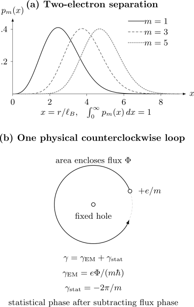
Top: normalized radial probabilities calculated from the two-electron Laughlin wavefunction for $m=1,3,5$. These are finite-pair distributions, not a calculation of the bulk $g(r)$. Bottom: moving a quasihole around another in the physical plane accumulates both an area-dependent electromagnetic phase and the statistical contribution $-2\pi/m$.

What the trial state proves and does not prove

At fractions where a screening Laughlin liquid is stable, this state gives a representative of the $\nu_0=1/m$ phase and is the exact densest zero-energy ground state of suitable short-range parent Hamiltonians. For a realistic Coulomb interaction, evidence comes from adiabatic continuity, numerical spectra, overlaps, entanglement structure, response, and experiments. A large finite-size overlap is valuable but is not by itself a thermodynamic proof of a phase: two states can have a small overlap yet share a phase, while a large overlap can obscure a gap closing outside the tested sizes.

Fractional Charge

A quasihole at physical position $(X,Y)$ has analytic coordinate $\eta=X-iY$. It is generated by one additional zero in every electron coordinate:

$$\Psi_{\mathrm{qh}}(\eta) = \prod_{i=1}^{N} \left( z_i-\eta \right) \Psi_m.$$

This state is still in the lowest Landau level. Inserting one electronic flux quantum adiabatically through the fluid gives the response estimate

$$\left|\Delta Q\right| = \left|\sigma_{xy}\right| \Phi_0 = \frac{1}{m} \frac{e^2}{h} \frac{h}{e} = \frac{e}{m}.$$

The missing electronic charge therefore gives the quasihole physical charge $+e/m$ relative to the background. A quasielectron has the opposite charge, but its lowest-Landau-level wavefunction is not obtained by merely replacing the holomorphic quasihole factor with an antiholomorphic one.

Fractional charge is charge carried by a collective excitation of the electron fluid. It does not mean that a microscopic electron has been divided into independently existing vacuum particles. Local operators create topologically neutral combinations, move charge to a boundary, or couple to quasiparticles already present.

How charge is measured

In a weak-backscattering regime where rare tunneling events are approximately independent, low-frequency excess noise approaches the Poisson form

$$S_I(0) \simeq 2e^\ast I_B, \qquad e^\ast V \gg k_B T,$$

where $I_B$ is the backscattered current. Experiments at $\nu=1/3$ found $e^\ast\simeq e/3$. Away from the dilute-event regime, bunching, energy-dependent transmission, edge reconstruction, and thermal noise can change the inferred effective charge. A fit parameter called $e^\ast$ must therefore be accompanied by its transport model and bias window.

Anyonic Statistics

In two spatial dimensions, exchanging identical particles is described by braids rather than only by permutations. For an Abelian Laughlin quasihole with the physical field and charge fixed above, a physical counterclockwise exchange contributes

$$R_{\mathrm{qh},\mathrm{qh}} = \exp\left( -\frac{i\pi}{m} \right),$$

while taking one quasihole all the way around another gives the full-braid phase

$$M_{\mathrm{qh},\mathrm{qh}} = R_{\mathrm{qh},\mathrm{qh}}^2 = \exp\left( -\frac{i2\pi}{m} \right).$$

Physical clockwise paths complex-conjugate these expressions. In the reflected $z$ plane, a counterclockwise braid instead has $R_z=e^{i\pi/m}$ and $M_z=e^{i2\pi/m}$. This is an orientation dictionary, not a change of the physical state. Exchange, full braid, and the Aharonov–Bohm phase from fractional electric charge are distinct contributions.

One direct sign check uses the normalized quasihole state. For well-separated holes deep in a screening Laughlin fluid, the squared norm $Z=\langle\Phi\vert\Phi\rangle$ of the unnormalized polynomial state has position dependence

$$\log Z =\frac{1}{2m\ell_B^2}\sum_a\lvert\eta_a\rvert^2 -\frac{1}{m}\sum_{a<b}\log\frac{\lvert\eta_a-\eta_b\rvert^2}{\ell_B^2} +\text{constant}.$$

This screening limit neglects separation and boundary corrections. With the inherited Berry connection $\mathcal A=i\langle\Psi\vert d\Psi\rangle$, holomorphic parameter dependence gives

$$\mathcal A =\frac{i}{2}\sum_a \left(\partial_{\eta_a}\log Z\,d\eta_a -\partial_{\bar\eta_a}\log Z\,d\bar\eta_a\right).$$

On a physical counterclockwise loop enclosing flux $\Phi$ and $N_{\mathrm{in}}$ other quasiholes, this yields

$$\gamma =\frac{e\Phi}{m\hbar} -\frac{2\pi}{m}N_{\mathrm{in}}.$$

The first term has the Aharonov–Bohm sign of charge $+e/m$; subtracting it leaves the statistical phase above. This is the normalized-state version of the Berry-transport argument of Arovas, Schrieffer, and Wilczek (1984); Tong (2016), Sec. 3.2.3, develops the screening calculation. Berry-connection and spatial-orientation conventions must both be translated when comparing sources.

For several localized quasiholes, the Berry phase accumulated around a closed path contains both an area-dependent electromagnetic term and a path-topological term. A schematic interferometer phase is

$$\varphi = 2\pi \frac{e^\ast}{e} \frac{\Phi}{\Phi_0} + 2\theta N_{\mathrm{in}} + \varphi_{\mathrm{dyn}},$$

For a physical counterclockwise Laughlin-quasihole path, $e^\ast=+e/m$, $\theta=-\pi/m$, and $N_{\mathrm{in}}$ counts enclosed quasiholes of the same type. Other enclosed types require their mutual braid phase. Device charging, edge motion, neutral modes, and bulk–edge coupling can alter the apparent periods and phase slips, so an interference pattern is interpreted through a calibrated device model.

For the $\nu_0=1/3$ state, Nakamura et al. (2020) measured interference phase slips and Bartolomei et al. (2020) measured collision-induced current correlations compatible with Abelian anyonic statistics in their specified device regimes. This does not settle the statistics of every observed fractional plateau. In particular, identifying non-Abelian order requires evidence beyond a fractional Hall coefficient or a fractional tunneling charge.

Composite Fermions

The Laughlin states explain $\nu=1/m$, but many observed odd-denominator fractions organize into the Jain sequences

$$\nu = \frac{n}{2pn\pm1}, \qquad n,p\in\mathbb N.$$

The composite-fermion construction binds $2p$ correlation vortices to each electron. At mean-field level the resulting fermions experience

$$B^\ast = B-2p n_e\Phi_0.$$

Defining their effective filling by $\nu^\ast=n_e\Phi_0/B^\ast$ gives, for the same effective-field orientation,

$$\frac{1}{\nu^\ast} = \frac{1}{\nu}-2p, \qquad \nu = \frac{\nu^\ast} {2p\nu^\ast+1}.$$

An integer quantum Hall state of composite fermions at $\nu^\ast=n$ then maps to $\nu=n/(2pn+1)$. Reversing the effective-field orientation produces the minus sequence.

For example,

$$\nu = \frac{2}{5} \quad\Longleftrightarrow\quad p=1, \qquad \nu^\ast=2.$$

This converts a difficult interacting-electron fraction into two filled effective Landau levels of emergent fermions, while the underlying electron wavefunction remains strongly correlated. At $\nu=1/2$ with $p=1$, the mean effective field vanishes:

$$B^\ast=0.$$

The resulting compressible composite Fermi liquid is not a gapped fractional Hall plateau. Pairing or other instabilities of composite fermions provide routes to even-denominator phases, but the resulting order depends on Landau level, interaction, symmetry, and particle–hole structure.

Flux attachment is field-theory and wavefunction language. The attached flux is not an additional microscopic magnetic field concentrated at each electron, and the mean-field cancellation does not remove gauge fluctuations. Composite fermions and hierarchy constructions are complementary organizations of fractional Hall states; universal equivalence must be checked through response, quasiparticle, edge, and ground-sector data.

Edge Modes

A gapped Hall bulk next to vacuum requires low-energy boundary structure. The minimal $\nu=1/m$ edge is one downstream chiral boson. Fix a right boundary with fluid at physical $x<0$ and vacuum at $x>0$, and let $s=+y$ increase along it. Downstream is then $-s$ for electrons at $B>0$. In units with $\hbar=1$, one consistent fixed-point action is

$$S_{\mathrm{edge}} = \frac{m}{4\pi} \int dt\,ds \left[ \partial_t\phi\,\partial_s\phi - v \left( \partial_s\phi \right)^2 \right].$$

Take $v>0$. The equation $\partial_t\phi=v\partial_s\phi$ propagates towards $-s$, as required. The charge density is

$$\rho(s) = \frac{e}{2\pi} \partial_s\phi.$$

The vertex operator $e^{il\phi}$ carries charge $le/m$: the equal-time algebra $[\phi(s),\phi(s^\prime)]=-i\pi\operatorname{sgn}(s-s^\prime)/m$ gives $[Q,e^{il\phi}]=(le/m)e^{il\phi}$. Thus $l=1$ creates a charge-$+e/m$ quasihole, $l=m$ creates a local electron hole (annihilates an electron), and $l=-m$ creates a charge-$-e$ electron. At this ideal single-mode fixed point, the vertex has scaling dimension $\Delta_l=l^2/(2m)$, so its zero-temperature correlation decays as $|t|^{-l^2/m}$. Weak electron tunneling from a normal Fermi-liquid contact therefore gives $I\propto V^m$ at positive bias. Weak quasihole tunneling between two such edges instead gives

$$I_B\propto V^{2/m-1}.$$

The latter is a perturbative result above the crossover to strong backscattering, with $e^*V\gg k_BT$ and energies below the bulk gap. For $m>2$ its negative exponent signals the breakdown of weak-backscattering perturbation theory as bias decreases; it does not predict an infinite physical current at zero bias (Wen, 1990; Chang, 2003).

Real edges can reconstruct into additional counterpropagating charged or neutral branches. Disorder and interactions can drive equilibration between branches, and a finite device may not reach the asymptotic edge fixed point over the available length or temperature range. Electrical conductance sees net charge transport; heat transport also sees neutral modes. The signed laboratory thermal Hall coefficient is

$$\begin{aligned} \frac{\kappa_{xy}}{T} &=c_{xy}\frac{\pi^2 k_B^2}{3h}, \\ c_{xy}&=-1 \quad\text{(Laughlin, $B>0$)}. \end{aligned}$$

Here $c_{xy}$ is the signed chiral coefficient in the declared physical heat tensor. The positive-chirality analytic-plane convention used for the $K$ matrix below has $c_z=\operatorname{signature}K=+1$, with $c_{xy}=-c_z$ under the reflection. These symbols prevent an orientation change from being hidden in the word “downstream.” At $m=1$, the negative thermal sign also agrees with the normal-state Wiedemann–Franz relation to $\sigma_{xy}<0$. For candidate even-denominator orders, electrical Hall response can agree while the chiral coefficient and neutral-mode content differ, making thermal and noise measurements especially sensitive to equilibration.

Topological Order

The fractional Hall effect is not only fractional conductivity. The $\nu=1/m$ Laughlin phase has a coherent package:

• a gap above the ground space and local indistinguishability within it;
• $m$ topological ground sectors on a torus, with splitting that vanishes at large size (typically exponentially for local gapped models);
• $m$ Abelian quasiparticle sectors;
• elementary charge magnitude $e/m$;
• exchange-angle magnitude $\pi/m$ for the elementary quasihole, with physical counterclockwise angle $-\pi/m$;
• a chiral boundary anomaly matching the bulk response;
• long-range entanglement.

To retain the familiar positive $K$ notation, the following compact Abelian description is oriented in the reflected analytic $z$ plane:

$$K=(m), \qquad t=(1).$$

Choose integer sector representatives $l=0,1,\ldots,m-1$. The positive filling and signed quasihole charge are

$$\nu = t^{\mathsf T}K^{-1}t = \frac{1}{m},$$ $$\frac{q_l}{e} = t^{\mathsf T}K^{-1}l = \frac{l}{m},$$

and

$$\theta_l^{(z)} = \pi l^{\mathsf T}K^{-1}l = \frac{\pi l^2}{m} \pmod{2\pi}.$$

The physical counterclockwise angle is $\theta_l^{(xy)}=-\theta_l^{(z)}$. Correspondingly, the laboratory responses are $\sigma_{xy}=-(e^2/h)t^{\mathsf T}K^{-1}t$ and $c_{xy}=-\operatorname{signature}K$. The $K$ matrix has not been partly reinterpreted as a physical-plane matrix.

For odd $m$, attaching a local electron or electron hole shifts $l$ by $\pm m$. It changes the exchange phase by $-1$ and the charge by a local integer charge, while leaving mutual braiding invariant. Thus an exchange phase modulo $2\pi$ is assigned to a chosen representative, not to $l\bmod m$ alone. A complete fermionic description retains the transparent local fermion and spin structure, as explained in Topological Order. These formulas summarize the topological data; they do not derive the microscopic phase or prove that a material realizes it.

Because every Laughlin sector has quantum dimension one,

$$\mathcal D = \sqrt{m}, \qquad \gamma = \ln\mathcal D = \frac12\ln m$$

for the vacuum-sector topological entanglement entropy. Topological Entanglement Entropy Preview explains subtraction geometries and finite-size limitations.

Many-body Chern response

Thread boundary twists $\theta_x,\theta_y$ through the physical $x,y$ cycles of a torus, with a many-electron wavefunction gaining $e^{i\theta_\mu}$ when one electron is moved through cycle $\mu$. Use $\mathcal A_\mu^{ab}=i\langle\Psi_a\vert\partial_{\theta_\mu}\Psi_b\rangle$ and the ordered twist orientation $d\theta_x\wedge d\theta_y$. If a locally indistinguishable ground space has dimension $q$, its non-Abelian Berry curvature has an integer first Chern number

$$C_{\mathcal G} = \frac{1}{2\pi} \int_0^{2\pi} d\theta_x \int_0^{2\pi} d\theta_y\, \operatorname{Tr} \mathcal F_{\theta_x\theta_y}.$$

For a ground-state multiplet isolated over the entire twist torus, the equal-sector, twist-averaged response is

$$\sigma_{xy} = -\frac{e^2}{h} \frac{C_{\mathcal G}}{q}.$$

The fixed-twist response approaches this average in the appropriate insulating thermodynamic limit. Arbitrary mixtures of accidentally degenerate states do not satisfy this conclusion. For the Laughlin state, $q=m$ and $C_{\mathcal G}=1$ give $\sigma_{xy}=-e^2/(mh)$ in the declared physical convention. The fractional coefficient therefore does not mean that a single noninteracting Bloch band has a fractional first Chern number. The integer belongs to the entire ground-state bundle; the denominator reflects its topological ground-space structure.

What each measurement can establish

Different measurements establish different parts of the phase:

Observation	Strongest direct inference	What it does not establish alone
Hall plateau with small $\rho_{xx}$	robust fractional transverse response	quasiparticle statistics or complete order
activated transport or compressibility jump	an incompressible regime and energy scale	universal gap or anyon content
shot-noise charge $e^\ast$	tunneling-event charge in a stated model	exchange statistics
interferometric phase slips	braiding-compatible phase information	interpretation without electrostatic calibration
collider correlations	exchange-statistics-sensitive correlations	arbitrary non-Abelian braid matrices
thermal Hall response	net chiral energy transport	microscopic wavefunction by itself
torus spectrum and flux flow in numerics	candidate topological sectors and response	thermodynamic phase without scaling
entanglement spectrum or entropy	universal-structure evidence under assumptions	complete anyon theory from one number

Agreement across transport, thermodynamics, quasiparticle charge, braiding-sensitive observables, edge structure, and finite-size scaling is more authoritative than any single diagnostic.

Beyond the simplest Laughlin liquid

Different orders can share a Hall coefficient. At half filling of an active Landau level, pairing of composite fermions can produce non-Abelian candidates with distinct neutral modes and quasiparticle data. Distinguishing them requires more than a rational Hall value or a fractional tunneling charge. Edge reconstruction and incomplete equilibration can complicate thermal and noise measurements even for a known bulk phase.

Lattice Chern bands provide another setting for interaction-driven fractionalization; their form factors and quantum geometry replace some of the special Landau-level structure. Fractional Quantum Hall Frontiers and Fractional Chern Insulators discuss current experiments and open identification problems. The general fusion and ground-state structure is developed in Topological Order.

Exercises

1. Filling and flux counting

A spin-resolved two-dimensional electron gas has density

$$n = 1.20\times10^{15}\ \mathrm{m}^{-2}.$$

At what magnetic field is $\nu=1/3$? Estimate $\ell_B$ there.

Solution

From $\nu=nh/(eB)$,

$$B = \frac{nh}{e\nu} = 3\frac{nh}{e} \simeq 14.9\ \mathrm T.$$

Then

$$\ell_B = \sqrt{\frac{\hbar}{eB}} \simeq 6.65\ \mathrm{nm}.$$

The calculation assumes one resolved spin and flavor component. An unresolved degeneracy would change the interpretation of the same density and field.

2. Pair probability and radial probability

For the two-electron state, explain why the probability per unit area vanishes as $r^{2m}$ but the radial density vanishes as $r^{2m+1}$. Find the maximum of $p_m(x)$ and its mean squared separation.

Solution

The amplitude contains $(z_1-z_2)^m$, and squaring gives $r^{2m}$. Integrating a thin annulus contributes its area $2\pi r\,dr$. Setting $d\log p_m/dx=(2m+1)/x-x/2=0$ gives $x_{\rm max}=\sqrt{4m+2}$. With $u=x^2/4$, the radial measure becomes $u^m e^{-u}du/m!$, whose mean is $m+1$. Hence

$$\langle r^2\rangle=4(m+1)\ell_B^2.$$

Odd $m$ is required for fermionic antisymmetry. The radial measure does not change that exchange property.

3. Flux transport and elementary charge at two fifths

In the positive analytic-plane convention, a simple Jain state has

$$K=\begin{pmatrix}3&2\\2&3\end{pmatrix}, \qquad \mathbf t=\begin{pmatrix}1\\1\end{pmatrix}.$$

Use the charge formula above to find the charge of sector $\mathbf l=(1,0)^{\mathsf T}$ and the charge transported by one flux quantum. Explain why they differ.

Solution

$$K^{-1}=\frac15\begin{pmatrix}3&-2\\-2&3\end{pmatrix}.$$

Thus $\mathbf t^{\mathsf T}K^{-1}\mathbf l=1/5$, whereas $\mathbf t^{\mathsf T}K^{-1}\mathbf t=2/5$. The elementary charge magnitude is $e/5$; one flux quantum transports magnitude $2e/5$. Flux insertion creates the sector represented by $\mathbf t$, not necessarily one elementary quasiparticle. Charges of all integer sectors are multiples of $e/5$, and a local electron changes charge by an integer multiple of $e$.

4. Which gap is being measured?

Suppose a Laughlin $1/3$ liquid has isolated quasielectron and quasihole creation energies $\epsilon_{\rm qe}$ and $\epsilon_{\rm qh}$. Neglect their interactions at large separation. Compare the elementary pair energy with the electron-addition chemical-potential jump at fixed flux. Does either equal the splitting of topological ground states on a large torus?

Solution

An elementary neutral pair costs $\epsilon_{\rm qe}+\epsilon_{\rm qh}$. Adding or removing one electron creates three elementary excitations of the appropriate charge, so after canceling the common chemical-potential and background contributions,

$$\Delta_c=3(\epsilon_{\rm qe}+\epsilon_{\rm qh}).$$

Binding, spin textures and finite-size electrostatics can alter this simple estimate. The torus ground-state splitting instead tends to zero while the excitation gaps remain finite. An Arrhenius transport gap requires its own mobility and disorder assumptions.

5. Edge tunneling at one third

At the ideal $m=3$ edge fixed point, compare the scaling dimensions of an electron and a quasihole. What do the two weak-tunneling predictions imply as bias is lowered?

Solution

The electron has $|l|=3$, hence $\Delta_e=3/2$; the quasihole has $l=1$, hence $\Delta_{\rm qh}=1/6$. A normal contact gives $I\propto V^3$. Quasihole transfer between two edges has total scaling dimension $1/3$, and its perturbative backscattered current scales as $V^{-1/3}$. The growing correction means the weak-backscattering description fails at low bias. Thermal rounding or the strong-backscattering regime must then replace that formula.

Further Reading

• B. I. Halperin and J. K. Jain, eds., Fractional Quantum Hall Effects: New Developments, World Scientific, 2020, surveys modern experiments, composite fermions, edges, and candidate non-Abelian phases.
• T. H. Hansson, M. Hermanns, S. H. Simon, and S. F. Viefers, “Quantum Hall Physics: Hierarchies and Conformal Field Theory Techniques,” Reviews of Modern Physics 89, 025005 (2017), doi:10.1103/RevModPhys.89.025005.
• J. K. Jain, Composite Fermions, Cambridge University Press, 2007, develops the wavefunctions, effective-field mapping, excitations, and phenomenology of the Jain sequence.
• C. Nayak, S. H. Simon, A. Stern, M. Freedman, and S. Das Sarma, “Non-Abelian Anyons and Topological Quantum Computation,” Reviews of Modern Physics 80, 1083–1159 (2008), doi:10.1103/RevModPhys.80.1083.

References

• D. Arovas, J. R. Schrieffer, and F. Wilczek, “Fractional Statistics and the Quantum Hall Effect,” Physical Review Letters 53, 722–723 (1984), doi:10.1103/PhysRevLett.53.722.
• H. Bartolomei et al., “Fractional Statistics in Anyon Collisions,” Science 368, 173–177 (2020), doi:10.1126/science.aaz5601.
• A. M. Chang, “Chiral Luttinger Liquids at the Fractional Quantum Hall Edge,” Reviews of Modern Physics 75, 1449–1505 (2003), doi:10.1103/RevModPhys.75.1449.
• R. de-Picciotto et al., “Direct Observation of a Fractional Charge,” Nature 389, 162–164 (1997), doi:10.1038/38241.
• F. D. M. Haldane, “Fractional Quantization of the Hall Effect: A Hierarchy of Incompressible Quantum Fluid States,” Physical Review Letters 51, 605–608 (1983), doi:10.1103/PhysRevLett.51.605.
• B. I. Halperin, “Statistics of Quasiparticles and the Hierarchy of Fractional Quantized Hall States,” Physical Review Letters 52, 1583–1586 (1984), doi:10.1103/PhysRevLett.52.1583.
• J. K. Jain, “Composite-Fermion Approach for the Fractional Quantum Hall Effect,” Physical Review Letters 63, 199–202 (1989), doi:10.1103/PhysRevLett.63.199.
• R. B. Laughlin, “Anomalous Quantum Hall Effect: An Incompressible Quantum Fluid with Fractionally Charged Excitations,” Physical Review Letters 50, 1395–1398 (1983), doi:10.1103/PhysRevLett.50.1395.
• J. Nakamura, S. Liang, G. C. Gardner, and M. J. Manfra, “Direct Observation of Anyonic Braiding Statistics,” Nature Physics 16, 931–936 (2020), doi:10.1038/s41567-020-1019-1.
• Q. Niu, D. J. Thouless, and Y.-S. Wu, “Quantized Hall Conductance as a Topological Invariant,” Physical Review B 31, 3372–3377 (1985), doi:10.1103/PhysRevB.31.3372.
• L. Saminadayar, D. C. Glattli, Y. Jin, and B. Etienne, “Observation of the $e/3$ Fractionally Charged Laughlin Quasiparticle,” Physical Review Letters 79, 2526–2529 (1997), doi:10.1103/PhysRevLett.79.2526.
• D. Tong, “Lectures on the Quantum Hall Effect,” lecture notes (2016), arXiv:1606.06687, Sec. 3.2.3 — normalized quasihole Berry transport and screening; translate the connection and path-orientation conventions explicitly.
• D. C. Tsui, H. L. Stormer, and A. C. Gossard, “Two-Dimensional Magnetotransport in the Extreme Quantum Limit,” Physical Review Letters 48, 1559–1562 (1982), doi:10.1103/PhysRevLett.48.1559.
• X.-G. Wen and Q. Niu, “Ground-State Degeneracy of the Fractional Quantum Hall States in the Presence of a Random Potential and on High-Genus Riemann Surfaces,” Physical Review B 41, 9377–9396 (1990), doi:10.1103/PhysRevB.41.9377.
• X.-G. Wen, “Chiral Luttinger Liquid and the Edge Excitations in the Fractional Quantum Hall States,” Physical Review B 41, 12838–12844 (1990), doi:10.1103/PhysRevB.41.12838.