Bulk–Boundary Correspondence

Bulk–boundary correspondence relates a difference between bulk phases to a feature of their interface that local changes cannot remove. For two-dimensional Chern insulators, that feature is the number of right-moving minus left-moving channels through the bulk gap. Extra pairs of channels may appear or disappear. In a finite strip, even the protected channels can mix with the opposite edge and acquire a small gap: the exact theorem concerns an isolated interface in the thermodynamic limit.

We first make the sign and channel count precise, then solve a lattice edge explicitly. The same example explains penetration depth, finite-width gaps and numerical checks. A Dirac mass wall and a flux-insertion argument give complementary physical explanations. Interacting and disordered systems require more general statements than counting electron bands.

Required background. Topology in Quantum Matter explains gapped phase equivalence and protecting symmetries.

Helpful background. Chern Numbers in Band Theory develops the occupied-band invariant; Tight-Binding Models explains real-space hopping matrices. For scattering and experiments on the resulting modes, see Edge and Surface States.

Bulk invariants and oriented boundary modes

Consider a local Hermitian Hamiltonian with an interface normal to $x$. The left bulk occupies $x<0$ and the right bulk $x>0$. Both are insulating at the same reference energy $E_F$. Translation along $y$ initially lets us label states by $k_y$. Use Berry connection $A_i=+i\langle u|\partial_{k_i}u\rangle$, Brillouin-zone orientation $dk_x\wedge dk_y$, and electron charge $-e$, with $e>0$.

Define the relative occupied-band Chern number

$$\Delta C=C_R-C_L.$$

At each crossing of $E_F$, a positive slope $\partial E/\partial k_y$ means motion in the positive $y$ direction. Call its contribution $+1$; a negative-slope crossing contributes $-1$. The net count is

$$\chi=N_{\mathrm R}-N_{\mathrm L}.$$

With these orientations, the bulk–boundary theorem states

$$\boxed{\chi=\Delta C.}$$

Here $N_{\mathrm R}$ and $N_{\mathrm L}$ count crossings, not distinct plotted curves. A curve can cross several times. At an accidental tangency, move $E_F$ slightly within the common gap or perturb the boundary infinitesimally so that the crossings are transverse. The stable result is independent of that choice (Hatsugai; Kellendonk, Richter and Schulz-Baldes; Graf and Porta).

For example, three positive and two negative crossings give $\chi=1$. Local boundary couplings can remove two counterpropagating pairs while leaving one channel. They cannot remove the last channel without changing the bulk mismatch or the assumptions of the theorem. Ordinary surface potentials can create additional in-gap states, so the mere presence of one localized state is a weaker statement.

The comparison always involves two phases. At a sample’s left edge, vacuum is on the left and the material on the right; if vacuum has $C=0$, then $\chi=C$. At the right edge, the order reverses and $\chi=-C$. Reversing coordinates requires transforming the Berry and propagation conventions together. A sign taken from a plot with unspecified axes cannot be compared reliably with a bulk invariant.

Other invariants count different boundary features

The Chern example is an integer index. Other symmetries change what remains invariant:

Bulk quantity	Boundary feature
Chern-number difference	Signed chiral crossings
One-dimensional chiral winding	Signed zero-mode count
Two-dimensional class-AII index	Kramers switching parity
Three-dimensional strong class-AII index	Odd surface-cone parity in band theory
Superconducting index	Majorana zero modes or spectral flow

For a chiral-symmetric chain, choose the chiral operator $\Gamma=\operatorname{diag}(I,-I)$ and write

$$H(k)=\begin{pmatrix}0&q(k)\\q^\dagger(k)&0\end{pmatrix}.$$

The winding is

$$\nu=\frac{1}{2\pi i}\int_{\mathrm{BZ}} \partial_k\log\det q(k)\,dk.$$

With the same right-minus-left spatial convention and Fourier convention $c_x\propto e^{ikx}$, the interface zero modes obey $N_+-N_-=\nu_L-\nu_R$, where $N_\pm$ count their $\Gamma$ eigenvalues. A pair of zero modes with opposite $\Gamma$ eigenvalues can hybridize into finite-energy states without changing this index. The SSH Model illustrates why the unit cell and termination must be specified together. Breaking chiral symmetry can shift a zero mode away from zero.

For a time-reversal-invariant class-AII insulator, the charge Chern number vanishes. An odd relative $\mathbb Z_2$ index instead forces odd Kramers partner switching. Additional trivial pairs do not change that parity. Weak and crystalline indices require a surface orientation and termination compatible with their protecting spatial symmetries; they do not require identical gaplessness on every surface. See Topological Insulators.

In a superconductor, count independent Majorana degrees of freedom with the BdG particle–hole constraint; counting each redundant electron/hole branch as a complex channel gives wrong thermal factors. A Weyl semimetal uses a different restriction: only its gapped two-dimensional momentum slices have the Chern edge theorem. Their modes join into Fermi arcs and delocalize at the node projections. The full three-dimensional bulk is gapless; see Topological Superconductors and Weyl and Dirac Semimetals.

A lattice edge that can be solved exactly

The two-band Qi–Wu–Zhang model makes the bulk invariant, edge direction and decay length calculable in one setting. Set the lattice spacing and hopping energy to one, and define

$$H(\mathbf k)=\sin k_x\,\sigma_x+\sin k_y\,\sigma_y +d_z(\mathbf k)\sigma_z,$$ $$d_z(\mathbf k)=M+\cos k_x+\cos k_y.$$

For the lower band in our Berry convention, $C=+1$ when $-2<M<0$, $C=-1$ when $0<M<2$, and $C=0$ when $|M|>2$. The gap closes at $M=-2,0,2$. These signs follow by summing the four regulated Dirac contributions, or independently by integrating the occupied-band curvature. The bulk computation is developed in Chern Numbers in Band Theory; here we test it using an open edge (Qi, Wu and Zhang; Mong and Shivamoggi).

From Bloch hopping to a half-space

Keep $k_y$ and open the lattice along $x$. Let

$$b=M+\cos k_y,$$ $$h_0=\sin k_y\,\sigma_y+b\sigma_z,$$ $$T=\frac{\sigma_z+i\sigma_x}{2}.$$

For cells $x=1,2,\ldots$, the Hamiltonian is

$$\widehat H=\sum_{x\ge1}c_x^\dagger h_0c_x +\sum_{x\ge1}(c_{x+1}^\dagger Tc_x+\mathrm{h.c.}).$$

The Fourier convention $c_x\propto e^{ik_xx}$ gives

$$e^{-ik_x}T+e^{ik_x}T^\dagger =\cos k_x\,\sigma_z+\sin k_x\,\sigma_x.$$

This reconstruction is a useful sign check before any diagonalization. A mistaken conjugation reverses the boundary direction.

Take the normalized spinor

$$\chi_+=\frac{1}{\sqrt2}\begin{pmatrix}1\\i\end{pmatrix}.$$

It satisfies $\sigma_y\chi_+=\chi_+$ and $T\chi_+=0$. The missing neighbor at $x=0$ is therefore compatible with an ansatz $\psi_x\propto\lambda^{x-1}\chi_+$. Substituting in the remaining terms gives

$$\lambda=-b, \qquad E_L(k_y)=\sin k_y.$$

The state exists only for $|b|<1$. Normalizing the geometric series yields

$$\psi_x=\sqrt{1-b^2}\,(-b)^{x-1}\chi_+.$$

The probability on the outermost cell is $1-b^2$. For $0<|b|<1$, its amplitude decay length, in lattice spacings, is

$$\xi=-\frac{1}{\log|b|}.$$

As $|b|\to1$, the normalized weight near the edge vanishes and $\xi$ diverges: the mode joins the projected bulk spectrum. At $b=0$, it is confined to the very first cell. This is an exact compact state; the decay-length formula has limiting value zero.

For $M=1.4$, the crossing occurs at $k_y=\pi$. Since $dE_L/dk_y=\cos k_y=-1$ there, the left edge has $\chi=-1$, in agreement with $C_R-C_L=-1-0$. The right edge has $E_R=-\sin k_y$ and opposite velocity. For $M=-1.4$, the left crossing is at $k_y=0$ with positive velocity, matching $C=+1$.

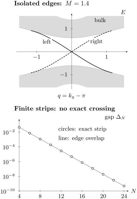
The lattice model at $M=1.4$. Top: solid and dashed curves are the left and right isolated-edge dispersions; gray regions are the projected bulk bands. At their endpoints the states cease to be normalizable edge modes. Bottom: circles show the gap at $k_y=\pi$ from finite-strip eigenvalues, and the line is the overlap estimate $2(1-0.4^2)0.4^N$. A nonzero gap at each finite width is consistent with gapless isolated edges as $N\to\infty$.

Finite strips and the order of limits

A strip of $N$ cells has two edges. Their low-energy modes can tunnel through the insulating interior. Near a crossing, their effective Hamiltonian has the form

$$H_{\mathrm{pair}}(q)=v_*q\,\tau_z+\delta_N\tau_x,$$

where $q$ is the momentum displacement, $v_*$ is the energy slope, and $\delta_N$ is the overlap matrix element. Thus

$$E_\pm(q)=\pm\sqrt{v_*^2q^2+\delta_N^2}.$$

At every finite $N$ with nonzero $\delta_N$, neither eigenvalue crosses zero. Exactly at the avoided crossing, the states can have equal weight on both edges. Assigning each such eigenstate to one edge by its mean position does not restore an exact crossing theorem.

The half-space correspondence is recovered by separating the boundaries before demanding arbitrarily fine energy resolution. Away from an exponentially narrow mixing region, a wide strip displays the two isolated-edge branches. The unlabelled total signed flow of a finite periodic family of matrices is zero, consistent with its two oppositely oriented boundaries.

The gap scale in the solvable model

At $k_y=\pi$ and $M=1.4$, put $b=M-1=0.4$. Changing to the $\sigma_y$ basis makes the finite-strip Hamiltonian off diagonal. Its positive energies are the singular values of an $N\times N$ matrix

$$B_{ij}=b\delta_{ij}+\delta_{j,i+1}.$$

The gap is $\Delta_N=2s_{\min}(B)$. In the wide-strip limit, overlap of the two geometric envelopes gives

$$\Delta_N\simeq2(1-b^2)|b|^N.$$

At $N=8$, the exact gap is approximately $1.1010\times10^{-3}$; at $N=16$, it is $7.2155\times10^{-7}$. Both are nonzero. Their rapid decrease reflects the same penetration length that appeared in the wavefunction. Exercise 3 extracts that length directly.

The prefactor is not universal. Additional valleys can produce oscillatory overlap, several decay lengths can coexist, and special parameters can give exact zeros. Here $M=1$, $k_y=\pi$ gives $b=0$: the two compact edge states have zero overlap at any width with distinct outer cells. A single vanishing gap, or a single small nonzero gap, therefore does not establish a general width law.

What to examine in a numerical spectrum

For each normalized eigenvector, inspect the cell probabilities $p_x=\|\psi_x\|^2$. Choose an edge window $x_c$ larger than the expected penetration depth but much smaller than $N$, and compute

$$w_L=\sum_{x=1}^{x_c}p_x, \qquad w_R=\sum_{x=N-x_c+1}^{N}p_x.$$

A mean position alone cannot distinguish a broad bulk state from a superposition of two edge states. Plot the profile or its spatial variance as well. Near a degeneracy, track the whole spectral subspace by overlap or projectors. Within a well-separated boundary subspace, diagonalizing the position operator can reveal localized combinations even when an eigensolver returns symmetric and antisymmetric states. These combinations need not be exact energy eigenstates of the finite strip.

Calculation	What it establishes
Refine bulk momentum mesh and check the gap	A stable occupied-band invariant
Reconstruct periodic hopping	The intended Bloch Hamiltonian and signs
Inspect edge probabilities	Spatial localization
Increase strip width	Separation of opposite edges
Vary boundary potentials	Stability of the limiting signed flow
Compare a second bulk algorithm	An independent numerical check

Count crossings at an energy in a common bulk gap. If a state overlaps the projected bulk continuum at the same momentum, generic coupling makes it a resonance rather than an isolated edge band; special symmetry-decoupled states need separate analysis. A surface spectral function can help identify such resonances, but its numerical broadening is not a physical lifetime. These tests complement, rather than replace, a bulk invariant.

A mass domain wall localizes a chiral channel

The lattice solution has a continuum counterpart. Let $v>0$, and write

$$H(k_y)=H_x+\hbar v k_y\sigma_y,$$ $$H_x=-i\hbar v\sigma_x\partial_x+m(x)\sigma_z.$$

Suppose $m(x)$ approaches $-m_0$ on the left and $+m_0$ on the right, with $m_0>0$. At $k_y=0$, multiply $H_x\psi=0$ by $\sigma_x$ and use $\sigma_x\sigma_z=-i\sigma_y$ to obtain

$$\partial_x\psi=-\frac{m(x)}{\hbar v}\sigma_y\psi.$$

For a $\sigma_y$ eigenvector $\chi_s$ with eigenvalue $s=\pm1$, integration gives

$$\psi_s(x)=\mathcal N e^{-sF(x)}\chi_s,$$ $$F(x)=\frac{1}{\hbar v}\int_0^x m(x')\,dx'.$$

The integral grows positively toward both spatial infinities, so only $s=+1$ decays on both sides. The momentum term acts on this state without changing its envelope:

$$E_0(k_y)=+\hbar vk_y.$$

Reversing the mass profile selects $s=-1$ and reverses the direction. This is the Jackiw–Rebbi domain-wall mechanism. The difference between regulated Dirac contributions agrees with the channel direction; a single unregulated continuum cone does not define an integer lattice Chern number. All high-momentum contributions and other valleys must be included when identifying the adjoining phases.

For a smooth wall, take

$$m(x)=m_0\tanh(x/\ell).$$

Define $a=m_0\ell/(\hbar v)$. Then $F(x)=a\log\cosh(x/\ell)$ and

$$\psi_0(x)\propto\operatorname{sech}^{a}(x/\ell)\chi_+.$$

Its far tails decay as $e^{-|x|/\xi}$ with $\xi=\hbar v/m_0$. The wall width $\ell$ controls its shape near the center; the asymptotic bulk gap controls the distant tails. A sufficiently smooth wall can also bind massive, nonchiral subbands, often called Volkov–Pankratov states. Their number depends on the profile, unlike the unpaired chiral branch (Tchoumakov and colleagues). Thus even this simple continuum example distinguishes the protected index from the raw number of bound states.

Two opposite-chirality modes can gap through a matrix that anticommutes with their kinetic term, as in $H_{\mathrm{pair}}$ above. A protecting symmetry may forbid that matrix. The same calculation also describes a line channel along a magnetic mass reversal on a topological-insulator surface: its two adjoining regions are gapped surface regions with different Hall responses, and the three-dimensional bulk supplies the anomalous surface setting.

Flux insertion and charge conservation

Why must a Chern insulator have boundary flow? Roll the sample into a cylinder, periodic along $y$ and open along $x$. Let positive flux mean $\Phi=\oint A_y\,dy$ along positive $y$. Inserting flux produces

$$E_y=-\frac{\dot\Phi}{L_y}.$$

With the stated electron and Berry conventions, the charge Hall conductivity is $\sigma_{xy}=-Ce^2/h$. Consequently the conventional charge current crossing the cylinder in positive $x$ is

$$I_x=L_y\sigma_{xy}E_y =C\frac{e^2}{h}\dot\Phi.$$

For one flux quantum $\Delta\Phi=h/e$, the transferred charge is

$$\Delta Q_x=Ce.$$

This is a charge sign: positive $C$ transfers negative electrons toward negative $x$. The flux cycle returns the bulk Hamiltonian to a gauge-equivalent form while moving charge between boundaries. Boundary states must accommodate that transfer; in band theory this appears as spectral flow through the chemical potential. Integer Quantum Hall Effect develops the transport geometry and mobility-gap version.

There is an order-of-limits condition. The insertion must be slow enough to avoid bulk excitations, but an isolated finite strip can have exponentially tiny avoided crossings between its edges. If a unique gapped finite-system ground state is followed adiabatically through all of these, a complete cycle returns its boundary charge distribution to the initial one. The usual transfer argument instead separates the edges first, or uses a process that is adiabatic for the bulk but effectively diabatic at their exponentially small mixing gaps. Reservoirs and relaxation define another physical occupation protocol; they must be stated when predicting a measurement.

For a two-level edge crossing with energy detuning $\varepsilon(t)$ and coupling $\delta_N$, the diabatic regime is parametrically

$$\hbar|\dot\varepsilon|\gg|\delta_N|^2.$$

An increasingly wide sample makes this compatible with slow bulk evolution. “Adiabatic insertion” without specifying the relevant gaps can therefore conceal an essential assumption.

Anomaly inflow and three different spectra

The response argument extends beyond free electrons. A chiral boundary treated alone appears to gain or lose charge under an applied electric field. The bulk Hall current supplies exactly that charge, so the complete system conserves it. This is anomaly inflow (Callan and Harvey). It states a consistency relation between bulk response and boundary physics, even when a one-electron quasiparticle is no longer a good description.

Do not confuse a physical energy spectrum with two useful bulk constructions. A Wilson-loop spectrum tracks occupied-state geometry and hybrid-Wannier positions. An entanglement spectrum tracks a reduced density operator across a virtual cut. Both may show related flow, but neither is by itself a measured energy dispersion or proof of a conducting physical surface. Boundary termination and interactions still matter.

Interactions and disorder change the boundary question

A gapped electron spectrum can still have an anomalous boundary

An interacting bulk invariant or quantized response constrains the whole boundary theory, not just its electron poles. A three-dimensional electronic topological insulator can have a gapless surface, break a protecting symmetry at the surface, or develop a symmetry-preserving surface with intrinsic topological order. The last possibility has fractional excitations and an anomalous symmetry action that an isolated two-dimensional system with the same microscopic symmetry cannot realize (Metlitski, Kane and Fisher; Wang, Potter and Senthil).

A fully gapped, symmetry-preserving, short-range-entangled surface with no such structure cannot terminate the nontrivial phase by itself. Coupling two boundaries with opposite anomalies can remove the obstruction, but changes the boundary system being considered. Interactions can also reduce a free-fermion classification; the surviving many-body invariant, explained in Symmetry-Protected Topological Phases, is the appropriate comparison.

Green-function formulas require care. A topological integer constructed from the one-electron Green function can change through a zero as well as a pole. A zero does not represent an electron excitation. Such a change need not imply a change of the actual interacting phase or of a quantized many-body response. The hypotheses connecting a particular Green-function invariant to the physical invariant must be checked; its mathematical pole/zero correspondence alone does not require a gapless electron spectrum (Gurarie; Essin and Gurarie).

Intrinsic topological order may allow a gapped edge

A nonchiral topologically ordered phase can have a fully gapped boundary when a suitable set of anyons can condense consistently, including any imposed symmetry constraints. Different condensates give different boundary types. Thus topological order does not automatically imply a conducting edge.

For a fixed two-dimensional phase, a nonzero physical chiral central charge $c_-$ obstructs a fully gapped boundary to vacuum. At an interface the relevant quantity is the difference of the two physical chiral central charges. Equality only modulo eight, as inferred from bosonic anyon data, is insufficient: adding an invertible chiral layer changes the thermal response and the interface problem. Conversely, zero difference is necessary but not generally sufficient for a gapped interface; compatible condensation data are also needed (Levin). See Topological Order.

When momentum is unavailable

Disorder removes the clean $E(k_y)$ plot, but not necessarily the phase. In a Hall insulator with the appropriate localization properties, a mobility gap can support a real-space Chern invariant and quantized edge response. The boundary statement uses current, scattering or localization rather than literal Bloch-band crossings (Bellissard, van Elst and Schulz-Baldes; Kellendonk, Richter and Schulz-Baldes).

A small density of states is not a demonstration of a mobility gap. Check localization and size dependence, vary disorder realizations, and compare bulk indices with a boundary response. Static local Hermitian results also cannot be transferred unchanged to non-Hermitian, driven or open-system models.

Why a finite sample’s local Chern marker sums to zero

A real-space diagnostic makes the role of the boundary especially visible. Let $P$ project onto occupied one-electron states and $Q=1-P$. Write $\operatorname{tr}_{\mathbf r}O$ for the sum of $\langle\mathbf r,\alpha|O|\mathbf r,\alpha\rangle$ over all orbitals $\alpha$ of one cell. For a lattice with cell area $A_c$, define

$$M_{\mathbf r}=\operatorname{tr}_{\mathbf r}(PXQYP),$$ $$\mathcal C(\mathbf r)=-\frac{4\pi}{A_c}\operatorname{Im}M_{\mathbf r}.$$

Here $X,Y$ are physical position operators, including orbital positions. The normalization matches our Berry convention. In a large clean sample, the marker deep in the interior approaches the bulk Chern number; in a disordered homogeneous region, an appropriate spatial average is used (Bianco and Resta).

For a finite open sample, however, the sum over all cells vanishes. The trace can be rearranged into the trace of a commutator of projected positions, which is zero in finite dimension. Boundary contributions compensate the interior. Averaging the whole flake therefore discards the quantity one intended to measure.

For example, at $M=1.4$, direct occupied-projector calculations on open $10\times10$, $14\times14$ and $18\times18$ square flakes give central four-cell averages approximately $-0.99447$, $-0.99982$ and $-0.99999$. Each whole-sample sum is zero to numerical precision. The bulk value $C=-1$ and the compensating boundary are consistent parts of the same calculation. Exercise 5 derives the sum rule.

Common pitfalls

A small strip gap proves the phase is trivial. Opposite-edge overlap gives a gap even when both isolated edges are topological. Check profiles and width dependence before interpreting it as a bulk change.

Every visible branch must survive. Only the appropriate signed count, parity or anomaly is protected. Trivial bands and smooth-wall massive subbands can disappear without changing it.

One continuum cone fixes an integer Chern number. Its mass reversal diagnoses a local transition; the full regulator fixes the integer and the relative sign.

No electron pole means no boundary constraint. Collective excitations, symmetry breaking and surface topological order can carry the interacting boundary structure. A Green-function zero is not an electron mode.

Exercises

1. Which channels can disappear?

An interface has $C_L=2$ and $C_R=-1$. Its spectrum shows two positive-slope and five negative-slope crossings in the common gap. Is it consistent with the theorem? Explain how many pairs can gap, and when a symmetry might forbid the proposed coupling.

Solution

Both counts give $-3$: $C_R-C_L=-3$ and $2-5=-3$. Two counterpropagating pairs can disappear, leaving three left-moving channels. For one pair,

$$H(q)=vq\tau_z+\mu\tau_x$$

has energies $E_\pm=\pm\sqrt{v^2q^2+\mu^2}$ because the two Pauli matrices anticommute. Its gap is $2|\mu|$ and its original net chirality was zero. If a required symmetry forbids the $\tau_x$ term, that pair cannot be removed by this coupling; one must analyze all symmetry-allowed perturbations.

2. Derive the exact lattice edge

Using $T\chi_+=0$, verify the left-edge solution, its normalization and the crossing direction for $M=1.4$. Find the range of $q=k_y-\pi$ in which it exists.

Solution

Since $T^\dagger\chi_+=\sigma_z\chi_+$, substituting $\psi_x=A\lambda^{x-1}\chi_+$ leaves the unwanted component proportional to $b+\lambda$. It vanishes at $\lambda=-b$, while the $\sigma_y$ component gives $E=\sin k_y$. The geometric norm is $|A|^2/(1-b^2)$, so $A=\sqrt{1-b^2}$.

For $M=1.4$,

$$b=1.4-\cos q, \qquad E_L=-\sin q.$$

The condition $|b|<1$ reduces to $\cos q>0.4$, hence

$$|q|<\arccos(0.4)\approx1.1593.$$

The slope at $q=0$ is $-1$, as required by the left-edge mismatch $\Delta C=-1$. At the two endpoints, $b=1$, the normalization weight at the edge vanishes and the mode joins the bulk continuum.

3. Extract a penetration length from finite gaps

At $M=1.4$, the gaps for widths 8 and 16 are $1.1010\times10^{-3}$ and $7.2155\times10^{-7}$. Estimate the amplitude penetration depth and compare it with the exact wavefunction. Does the absence of an exact zero crossing at either width contradict the theorem?

Solution

From $\Delta_N\propto e^{-N/\xi}$,

$$\xi=\frac{16-8}{\log(\Delta_8/\Delta_{16})} \approx1.0914$$

in lattice spacings. The exact isolated-edge envelope has $|\lambda|=0.4$, giving $\xi=-1/\log0.4\approx1.0914$. The agreement identifies the overlap scale. Neither finite strip has an exact zero crossing, but the gap vanishes as the two edges separate, which is the relevant limit.

4. A smooth wall and its penetration depth

For $m(x)=m_0\tanh(x/\ell)$, derive the localized zero-mode envelope and its dispersion. Compare widening the wall at fixed $m_0$ with reducing $m_0$ at fixed wall width. Which change increases the asymptotic penetration depth?

Solution

Write the mass integral as $I(x)=\int_0^x m(x')\,dx'$. It evaluates to

$$I(x)=m_0\ell\log\cosh(x/\ell).$$

It is positive at either infinity, so the normalizable spinor has $\sigma_y=+1$. Thus

$$\psi_0\propto\operatorname{sech}^{a}(x/\ell)\chi_+,$$

where $a=m_0\ell/(\hbar v)$, and $E_0=\hbar vk_y$. Its tails have length $\hbar v/m_0$, independently of the wall’s central shape.

Increasing $\ell$ at fixed $m_0$ broadens the central part of the profile but leaves the far-tail length unchanged. Reducing $m_0$ increases $\xi=\hbar v/m_0$ and weakens bulk confinement. Near the center, $\log\cosh(x/\ell)\simeq x^2/(2\ell^2)$, so the envelope is approximately Gaussian with width parameter $\sqrt{\hbar v\ell/m_0}$. Central width and asymptotic decay length are different quantities.

5. The marker’s boundary compensation

For a finite open sample, show that the cell sum of $\mathcal C(\mathbf r)$ vanishes even when its interior approaches a nonzero integer. Use $P^2=P$, $Q=1-P$ and $[X,Y]=0$.

Solution

The full trace satisfies

$$\operatorname{Tr}(PXQYP) =\operatorname{Tr}(PXY P) -\operatorname{Tr}(PXPYP).$$

The first term is real because $XY$ is Hermitian. With $\widetilde X=PXP$ and $\widetilde Y=PYP$, the imaginary part of the second is

$$\begin{aligned} \operatorname{Im}\operatorname{Tr}(\widetilde X\widetilde Y) &=\frac{1}{2i}\operatorname{Tr}[\widetilde X,\widetilde Y] \\&=0. \end{aligned}$$

The final equality uses finite-dimensional trace cyclicity. Therefore the total marker is zero. An interior average can still approach $C$ because the boundary values compensate it. One must take a bulk-region limit, not the whole finite-sample trace, to recover the bulk invariant.

References

• J. Bellissard, A. van Elst, and H. Schulz-Baldes, “The Noncommutative Geometry of the Quantum Hall Effect,” Journal of Mathematical Physics 35, 5373–5451 (1994), doi:10.1063/1.530758.
• R. Bianco and R. Resta, “Mapping Topological Order in Coordinate Space,” Physical Review B 84, 241106(R) (2011), doi:10.1103/PhysRevB.84.241106.
• C. G. Callan, Jr. and J. A. Harvey, “Anomalies and Fermion Zero Modes on Strings and Domain Walls,” Nuclear Physics B 250, 427–436 (1985), doi:10.1016/0550-3213(85)90489-4.
• A. M. Essin and V. Gurarie, “Bulk–Boundary Correspondence of Topological Insulators from Their Respective Green’s Functions,” Physical Review B 84, 125132 (2011), doi:10.1103/PhysRevB.84.125132.
• G. M. Graf and M. Porta, “Bulk–Edge Correspondence for Two-Dimensional Topological Insulators,” Communications in Mathematical Physics 324, 851–895 (2013), doi:10.1007/s00220-013-1819-6.
• V. Gurarie, “Single-Particle Green’s Functions and Interacting Topological Insulators,” Physical Review B 83, 085426 (2011), doi:10.1103/PhysRevB.83.085426.
• Y. Hatsugai, “Chern Number and Edge States in the Integer Quantum Hall Effect,” Physical Review Letters 71, 3697–3700 (1993), doi:10.1103/PhysRevLett.71.3697.
• R. Jackiw and C. Rebbi, “Solitons with Fermion Number 1/2,” Physical Review D 13, 3398–3409 (1976), doi:10.1103/PhysRevD.13.3398.
• J. Kellendonk, T. Richter, and H. Schulz-Baldes, “Edge Current Channels and Chern Numbers in the Integer Quantum Hall Effect,” Reviews in Mathematical Physics 14, 87–119 (2002), doi:10.1142/S0129055X02001107.
• M. Levin, “Protected Edge Modes without Symmetry,” Physical Review X 3, 021009 (2013), doi:10.1103/PhysRevX.3.021009.
• M. A. Metlitski, C. L. Kane, and M. P. A. Fisher, “Symmetry-Respecting Topologically Ordered Surface Phase of Three-Dimensional Electron Topological Insulators,” Physical Review B 92, 125111 (2015), doi:10.1103/PhysRevB.92.125111.
• R. S. K. Mong and V. Shivamoggi, “Edge States and the Bulk–Boundary Correspondence in Dirac Hamiltonians,” Physical Review B 83, 125109 (2011), doi:10.1103/PhysRevB.83.125109.
• X.-L. Qi, Y.-S. Wu, and S.-C. Zhang, “Topological Quantization of the Spin Hall Effect in Two-Dimensional Paramagnetic Semiconductors,” Physical Review B 74, 085308 (2006), doi:10.1103/PhysRevB.74.085308.
• S. Tchoumakov, V. Jouffrey, A. Inhofer, E. Bocquillon, B. Plaçais, D. Carpentier, and M. O. Goerbig, “Volkov–Pankratov States in Topological Heterojunctions,” Physical Review B 96, 201302(R) (2017), doi:10.1103/PhysRevB.96.201302.
• C. Wang, A. C. Potter, and T. Senthil, “Gapped Symmetry Preserving Surface State for the Electron Topological Insulator,” Physical Review B 88, 115137 (2013), doi:10.1103/PhysRevB.88.115137.

Further reading

• C.-K. Chiu, J. C. Y. Teo, A. P. Schnyder, and S. Ryu, “Classification of Topological Quantum Matter with Symmetries,” Reviews of Modern Physics 88, 035005 (2016), doi:10.1103/RevModPhys.88.035005.
• E. Prodan and H. Schulz-Baldes, Bulk and Boundary Invariants for Complex Topological Insulators: From K-Theory to Physics, Springer (2016), doi:10.1007/978-3-319-29351-6.