Berry-Phase Polarization and Charge Pumping

The dipole moment of a chosen crystal cell is not, by itself, the bulk electric polarization of an infinite periodic solid. Charges can be reassigned across a cell boundary without changing the crystal, and occupied Bloch states are extended rather than attached to unique cells. The physically appropriate bulk object is therefore an equivalence class of polarization values, together with changes tracked along a specified insulating path.

Berry-phase polarization joins the ionic charge positions to the holonomy of the complete occupied electronic subspace. It is defined modulo a polarization quantum. When an insulating Hamiltonian executes a closed, charge-conserving adiabatic cycle, a continuous polarization branch can wind by an integer number of quanta. That winding is a Chern number and measures the charge transported across the sample.

Required background. You should be able to identify a fixed-rank occupied Bloch subspace and use the convention $\mathcal A=+i\langle u|\partial u\rangle$. Bloch’s Theorem supplies the Brillouin-zone and reciprocal-sewing conventions, while Berry Connection supplies the gauge transformation law.

Helpful background. Conventions for Quantum Matter fixes charge, cell, and origin language. Zak Phase Preview provides one-dimensional holonomy intuition, and Wannier Functions explains localized frames and their obstructions. Before using the pump sections, review Adiabatic Approximation as a Method. Projectors is a useful compact review of the occupied-subspace algebra used below.

Polarization of a periodic crystal

Start with one positive ion of charge $+e$ at $\tau$ and one occupied electron center at $\bar x$ in a one-dimensional cell of length $a$. Their dipole per cell length is

$$P=\frac{e}{a}(\tau-\bar x).$$

Moving the chosen electron center from $\bar x$ to $\bar x+a$ describes the same periodic charge distribution but changes this representative by $-e$. Thus $P$ has units of charge in one dimension and is defined modulo $e$. A common change of origin shifts both positions equally and cancels in the neutral total. This elementary example explains why bulk polarization needs both ions and electrons, and why a polarization change requires a continuous path between states (King-Smith and Vanderbilt, 1993).

Below, electrons have charge $-e$, with $e>0$; spin states are counted explicitly, without an implicit factor of two. Lattice vectors and orbital positions are fixed unless stated otherwise. The ground state is an insulator with a fixed number of occupied bands. Crossings within the occupied set are allowed; a gap separating that set from empty states must remain open. A direct gap alone is insufficient for an insulating filling if valence and conduction extrema overlap at different momenta.

Electronic Polarization from an Occupied Subspace

Write the Bloch states as

$$|\psi_{n\mathbf k}\rangle = e^{i\mathbf k\cdot\mathbf r} |u_{n\mathbf k}\rangle,$$

with cell-periodic spinors normalized in the declared cell convention. Collect an orthonormal frame for the $N_{\mathrm{occ}}$ occupied states into $U(\mathbf k)$. The occupied projector is

$$P(\mathbf k) = U(\mathbf k)U^\dagger(\mathbf k).$$

It is unchanged by $U\mapsto UV$ for any $V(\mathbf k)\in U(N_{\mathrm{occ}})$, so it remains well defined when individual occupied eigenvectors cross or exchange labels. The frame’s non-Abelian Berry connection is

$$[\mathcal A_i(\mathbf k)]_{mn} = i\langle u_{m\mathbf k}|\partial_{k_i}u_{n\mathbf k}\rangle_c.$$

Changing the occupied frame by $U(\mathbf k)\mapsto U(\mathbf k)V(\mathbf k)$, with $V\in U(N_{\mathrm{occ}})$, gives

$$\mathcal A_i \mapsto V^\dagger\mathcal A_iV + iV^\dagger\partial_{k_i}V.$$

Individual diagonal connections and energy-sorted band labels are therefore not reliable at occupied-band crossings. The total occupied projector and the trace holonomy are the correct objects.

In one dimension, include the reciprocal endpoint sewing and define

$$\gamma_{\mathrm{occ}} = \oint_{\mathrm{BZ}} dk\, \operatorname{Tr}\mathcal A_k \pmod{2\pi}.$$

For a forward mesh $k_0,k_1,\ldots,k_N=k_0+G$, form overlap matrices

$$[M_j]_{mn} = \langle u_m(k_j)|u_n(k_{j+1})\rangle_c.$$

The final state must be the representative sewn back to the initial fiber. A stable numerical Wilson loop uses the unitary polar factors

$$\begin{aligned} \widetilde M_j&=M_j(M_j^\dagger M_j)^{-1/2},\\ \mathcal W&=\widetilde M_0\widetilde M_1\cdots\widetilde M_{N-1}. \end{aligned}$$

With the connection and forward-link convention used here,

$$\gamma_{\mathrm{occ}} = -\operatorname{Arg}\det\mathcal W \pmod{2\pi}.$$

The sign follows directly: a forward overlap is $1-i\mathcal A_k\,dk+O(dk^2)$. Reversing the loop or defining links in the opposite direction changes the corresponding sign convention.

Under a sewn occupied-frame change, $\mathcal W$ transforms by conjugation at the base point. Its determinant and unordered eigenvalue set are invariant. Across a parameter path, Wilson eigenphases may cross and permute; follow the subspace or the full center set continuously rather than sorting principal values independently at each step.

Orbital positions are part of the calculation

A vector of tight-binding coefficients is not always the full cell-periodic wavefunction. Write $|u_n\rangle=\sum_\alpha|\phi_{\alpha k}\rangle c_{\alpha n}$ in an orthonormal orbital frame and define its connection $[\mathcal A_k^{\rm orb}]_{\alpha\beta} =i\langle\phi_{\alpha k}|\partial_k\phi_{\beta k}\rangle$. The physical occupied connection is

$$\mathcal A_k =i c^\dagger\partial_k c +c^\dagger\mathcal A_k^{\rm orb}c.$$

For ideal point orbitals at fixed positions $\tau_\alpha$, using Bloch sums with phase $e^{ikR}$ gives $\mathcal A_k^{\rm orb}=\operatorname{diag}(\tau_\alpha)$. The second term is the within-cell dipole. General orbitals can also have off-diagonal position matrix elements. Alternatively, compute overlaps of the full cell-periodic states, including the basis overlaps and reciprocal sewing; then this contribution is already present. Adding it again would double count.

Changing representation consistently leaves physical predictions unchanged. Moving orbitals while holding only a coefficient Hamiltonian fixed changes the physical embedding and can change polarization. Likewise, omitting the within-cell term defines a different intermediate polarization, although its complete-cycle winding agrees when that omitted term returns to its initial value (Watanabe and Oshikawa, 2018).

Add Ions and Identify the Polarization Quantum

For $e>0$, the one-dimensional electronic polarization per transverse cell is

$$P_{\mathrm{el}} = -\frac{e}{2\pi}\gamma_{\mathrm{occ}} \pmod e.$$

It is modulo $e$, not modulo $e/a$. In $d$ dimensions, for a globally smooth, reciprocally sewn occupied frame in a fixed cell,

$$\mathbf P_{\mathrm{el}} = -\frac{e}{(2\pi)^d} \int_{\mathrm{BZ}} d^d k\, \operatorname{Tr}\boldsymbol{\mathcal A}(\mathbf k).$$

Each explicitly included occupied spinor contributes once. A calculation that uses spinless spatial orbitals to represent two exactly degenerate occupied spin states must state and insert the factor of two.

The ionic contribution is

$$\mathbf P_{\mathrm{ion}} = \frac{e}{\Omega_c} \sum_\kappa Z_\kappa\boldsymbol\tau_\kappa,$$

so the total is

$$\mathbf P = \mathbf P_{\mathrm{ion}} + \mathbf P_{\mathrm{el}}.$$

Moving one electron center by a lattice vector does not change the infinite crystal, but it changes the representative by

$$\mathbf P_q(\mathbf R) = \frac{e\mathbf R}{\Omega_c}.$$

Consequently,

$$\mathbf P \sim \mathbf P + \frac{e\mathbf R}{\Omega_c}.$$

For particles of another conserved charge, replace $e$ by the charge quantum appropriate to the transported species and state the sign. Ionic and electronic pieces separately depend on origin and cell assignment. For a neutral cell, their origin shifts cancel in the total. Reassigning whole charges between neighboring cells still changes the displayed representative by a polarization quantum.

The full-dimensional expression also assumes that the relevant occupied bundle admits the needed smooth sewing. A static Chern insulator has no global smooth periodic frame, so a naive bulk polarization vector built from that formula is not licensed. Hybrid Wannier centers or slice-resolved quantities may remain meaningful, but their direction and boundary conditions must be specified.

Wilson Loops, Wannier Centers, and Boundary-Charge Limits

When localized Wannier functions exist, the electronic polarization has the equivalent center representation

$$\mathbf P_{\mathrm{el}} = -\frac{e}{\Omega_c} \sum_{n=1}^{N_{\mathrm{occ}}} \overline{\mathbf r}_n \pmod{\frac{e\mathbf R}{\Omega_c}}.$$

In one dimension,

$$\sum_n\overline x_n = \frac{a}{2\pi}\gamma_{\mathrm{occ}} \pmod a.$$

This is a representation of the occupied charge center, not a statement that each individual Wannier center is an observable. The centers of an arbitrary Wannier basis can change under occupied-frame rotations. In contrast, the unordered eigenphases of a fixed Wilson loop are gauge invariant. In one dimension they give the centers of the corresponding projected-position eigenstates, modulo lattice translations. Wannier Functions explains localization, gauge choice, and obstruction theory. Wannierization Workflows explains numerical construction and the checks needed before using an interpolated position or velocity operator.

For a two-dimensional band structure, a Wilson loop along $k_x$ at fixed $k_y$ produces hybrid centers $\overline x_a(k_y)$. Their unordered flow can diagnose a Chern obstruction or a symmetry-protected pattern. That flow is not an extra set of electron trajectories. It is a gauge-invariant spectrum of an occupied-subspace holonomy.

Polarization constrains boundary charge only after the boundary is declared. For an insulating interface with normal $\mathbf n$ directed from region 1 to region 2,

$$\sigma_{\mathrm b} = (\mathbf P_1-\mathbf P_2)\cdot\mathbf n$$

modulo the charge per surface primitive cell. An outer surface is the special case with vacuum polarization chosen as the reference. Changing termination can add an integer surface charge; reconstruction, metallic surface bands, adsorbates, defects, electrodes, and mobile screening charge can change the measured value. Bulk polarization therefore does not predict an absolute end charge without specifying the termination and mobile screening charge.

Track Polarization Along a Gapped Path

Let an insulating Hamiltonian depend continuously on $\lambda\in[0,1]$. The fixed-rank occupied subspace must remain separated from empty states, and the physical filling must remain insulating, along the complete path. Define

$$\mathcal F_{k_i\lambda} = \partial_{k_i}\mathcal A_\lambda - \partial_\lambda\mathcal A_{k_i} - i[\mathcal A_{k_i},\mathcal A_\lambda].$$

At fixed lattice vectors, the electronic change is

$$\Delta P_{\mathrm{el},i} = \frac{e}{(2\pi)^d} \int_0^1 d\lambda \int_{\mathrm{BZ}}d^d k\, \operatorname{Tr}\mathcal F_{k_i\lambda}.$$

Add the ionic displacement on the same continuous branch. If the cell itself changes, use reduced polarization coordinates and distinguish proper from improper strain responses; the fixed-cell expression above is not sufficient.

Endpoint Berry phases alone do not select the branch of $\Delta\mathbf P$. Sample the path densely enough that neighboring representatives can be joined continuously, inspect occupied-subspace overlaps and the minimum gap, and add or subtract polarization quanta only to preserve that continuity. A nearest-branch rule is unsafe if one step can move by more than half a quantum; refine the path instead.

For a spatially uniform bulk at fixed geometry, charge conservation gives

$$\mathbf J(t) = \frac{d\mathbf P}{dt}, \qquad \Delta\mathbf P = \int_{t_i}^{t_f}dt\,\mathbf J(t).$$

This relation is why switching current can determine a polarization change. It does not turn a leaky terminal-current trace directly into bulk polarization: capacitive background, free-carrier conduction, electrode screening, domain fractions, and incomplete switching require a forward model.

A Closed Adiabatic Cycle Pumps Charge

Now let a translation-invariant one-dimensional electronic Hamiltonian depend cyclically on $\lambda\in[0,2\pi]$:

$$H(k,\lambda+2\pi) = H(k,\lambda).$$

Before applying the result, require conserved $U(1)$ charge, fixed filling and occupied rank, a gap for every $(k,\lambda)$, and adiabatic following. Hold the ionic coordinates fixed for the displayed electronic theorem, or track their current separately. Orient the parameter torus by $dk\wedge d\lambda$ and define

$$C_{k\lambda} = \frac{1}{2\pi} \int_0^{2\pi}d\lambda \int_{\mathrm{BZ}}dk\, \operatorname{Tr}\mathcal F_{k\lambda}.$$

This is an integer for the continuous occupied bundle over the torus. With the electron and orientation conventions fixed above, the electronic contribution to conventional positive charge transported toward $+x$ in one cycle is

$$Q_{\mathrm{el},+x} = eC_{k\lambda}.$$

The sign follows from $P_{\mathrm{el}}=-e\int\mathcal A_k/(2\pi)$ and $\int\mathcal F_{k\lambda}=-\partial_\lambda\int\mathcal A_k$ after the $k$-boundary term is sewn away. Defining $\mathcal F_{\lambda k}$, reversing the torus orientation, or asking for electron rather than conventional-charge transport reverses the displayed sign. For $C_{k\lambda}=+1$, the aggregate electronic center flow is by $-a$, while conventional charge $+e$ moves toward $+x$.

The Hamiltonian returns to itself, so the endpoint polarization classes agree. The continuously unwrapped branch need not return to the same representative:

$$P_{\mathrm{el}}(2\pi) = P_{\mathrm{el}}(0) + eC_{k\lambda}$$

in the one-dimensional convention. If ions move, the total change is

$$\Delta P_{\mathrm{total}} = eC_{k\lambda} + \Delta P_{\mathrm{ion}}.$$

A closed structural cycle can carry an additional ionic polarization quantum. The branch winding, rather than a supposedly absolute endpoint polarization, is the pump invariant. A generic static Zak phase is neither quantized nor a Chern number.

The continuous Brillouin-zone integral describes the infinite periodic band system. On a finite ring, the charge integrated at one fixed boundary twist can vary continuously. Twist averaging recovers the Chern number, while equality at one fixed twist requires a thermodynamic-limit or twist-insensitivity argument.

Exact quantization is an adiabatic filled-state statement. Finite drive rate, thermal excitations, gap inhomogeneity, particle loss, coupling to reservoirs, and imperfect cycle closure produce platform-dependent corrections. Do not attach a universal error bar merely from the minimum gap; validate convergence with cycle time and inspect the actual transition channels.

For an open finite chain, topological pumping generally appears through edge spectral flow or exponentially small edge avoided crossings. Following one unique isolated open-system ground state around the full cycle is not the same theorem as the periodic bulk Chern number. State whether edge occupations are reset by reservoirs, followed diabatically across tiny edge gaps, or measured as accumulated boundary charge.

Symmetry Can Quantize a Polarization Class

A symmetry quantizes polarization only if it maps the declared state and charge distribution back to themselves while constraining the polarization class. In one dimension, inversion sends

$$P \mapsto -P \pmod e.$$

An inversion-symmetric gapped state therefore satisfies

$$P = 0 \quad\text{or}\quad \frac e2 \pmod e.$$

The claim concerns the total ionic plus electronic polarization, with an inversion center, origin, cell, and filling declared. The electronic SSH Zak phase can be $0$ or $\pi$ in a symmetry-compatible convention, but changing orbital embedding or unit cell changes its representative. The ionic reference and boundary termination are still required before inferring end charge.

Time reversal alone does not quantize ordinary electric polarization in one dimension because electric polarization is even under time reversal. Mirrors and rotations can constrain selected components, while nonsymmorphic or magnetic symmetries require their complete spatial and antiunitary actions. Symmetry of Bloch States explains those symmetry representations.

A quantized Thouless pump does not need a point symmetry at each intermediate time. Its integer follows from charge conservation, cyclicity, the gap, and the Chern class over the complete cycle. Symmetry can constrain endpoints or parts of a cycle, but it is not a substitute for those pump conditions.

Interacting, Disordered, and Finite-System Extensions

Crystal momentum is unavailable in a disordered sample, and a generic interacting ground state is not a list of occupied one-particle bands. On a one-dimensional periodic system of length $L$, let $\hat X=\sum_j\hat x_j$ denote the coordinate sum only inside the large-gauge exponential

$$\hat U_X = \exp\!\left( \frac{2\pi i}{L}\hat X \right).$$

The bare $\hat X$ is not a single-valued position observable on the periodic ring; $\hat U_X$ is the well-defined periodic operator.

For a localized insulating state with $z=\langle\Psi|\hat U_X|\Psi\rangle\ne0$, an electronic polarization representative is

$$P_{\mathrm{el}} = -\frac{e}{2\pi} \operatorname{Im}\log z \pmod e.$$

Add the ionic contribution and follow a continuous branch. A nonzero value of $z$ in one small finite system does not by itself prove a thermodynamic insulating phase; study size scaling, the charge gap or localization criterion, and sensitivity to boundary twists.

For an interacting or disordered pump, impose a boundary twist $\theta\in[0,2\pi]$ and a cyclic parameter $\lambda$. If a unique many-body ground state remains separated by a gap over the complete $(\theta,\lambda)$ torus, set

$$\mathcal A_\mu^{\mathrm{MB}} = i\langle\Psi(\theta,\lambda)| \partial_\mu\Psi(\theta,\lambda)\rangle,$$

and

$$\mathcal F_{\theta\lambda}^{\mathrm{MB}} = \partial_\theta\mathcal A_\lambda^{\mathrm{MB}} - \partial_\lambda\mathcal A_\theta^{\mathrm{MB}}.$$

Orient the torus by $d\theta\wedge d\lambda$ and define

$$C_{\mathrm{MB}} = \frac{1}{2\pi} \int_0^{2\pi}d\lambda \int_0^{2\pi}d\theta\, \mathcal F_{\theta\lambda}^{\mathrm{MB}}.$$

Then $eC_{\mathrm{MB}}$ is the boundary-twist-averaged geometric transported charge in the matching orientation convention. At a fixed twist, a finite ring can also carry an equilibrium persistent current. Subtract that current when identifying the pump contribution; its integral need not be quantized and can grow with the cycle duration. Its twist average vanishes because the ground-state energy is periodic in the twist. Pumped charge at one fixed twist approaches that value only with thermodynamic twist insensitivity; verify its size and twist dependence. Degenerate ground-state manifolds, fractional pumps, open-system steady states, and nonconserved charge require a different non-Abelian or dynamical statement; do not force them into the unique-ground-state formula. Boundary Conditions on Lattices explains the twist construction.

A Rice–Mele cycle, step by step

Consider a spinless chain with one occupied band and a rigid neutralizing ionic background. In the cell-periodic coefficient convention, let

$$H(k,\lambda)=\mathbf d\cdot\boldsymbol\sigma,$$ $$\begin{aligned} d_x&=t_1+t_2\cos(ka),\\ d_y&=t_2\sin(ka),\qquad d_z=\Delta,\\ t_1&=1+0.2\cos\lambda,\\ t_2&=1-0.2\cos\lambda,\\ \Delta&=0.4\sin\lambda. \end{aligned}$$

Energies are in units of the mean hopping. The band energies are $E_\pm=\pm|\mathbf d|$. Since $t_1,t_2>0$, the smallest separation occurs at $ka=\pi$:

$$\begin{aligned} \Delta_{\rm band}(\lambda) &=2\sqrt{(t_1-t_2)^2+\Delta^2}\\ &=0.8. \end{aligned}$$

The loop surrounds the degeneracy $(t_1-t_2,\Delta)=(0,0)$ without touching it. Follow $\lambda$ from $0$ to $2\pi$ and orient the torus by $dk\wedge d\lambda$. The lower-band curvature is

$$\mathcal F_{k\lambda} =\frac{\mathbf d\cdot (\partial_k\mathbf d\times\partial_\lambda\mathbf d)} {2|\mathbf d|^3}.$$

Its integral gives $C_{k\lambda}=-1$. Equivalently, the continuously followed forward-overlap phase falls by $2\pi$, so $\Delta P_{\rm el}=-e$: electrons move one cell toward $+x$, and conventional charge flows toward $-x$. Reversing the cycle reverses both statements. A loop shrunk to a point without crossing the degeneracy has zero winding. A path that crosses the degeneracy does not satisfy the gapped adiabatic-pump theorem (Rice and Mele, 1982; Thouless, 1983).

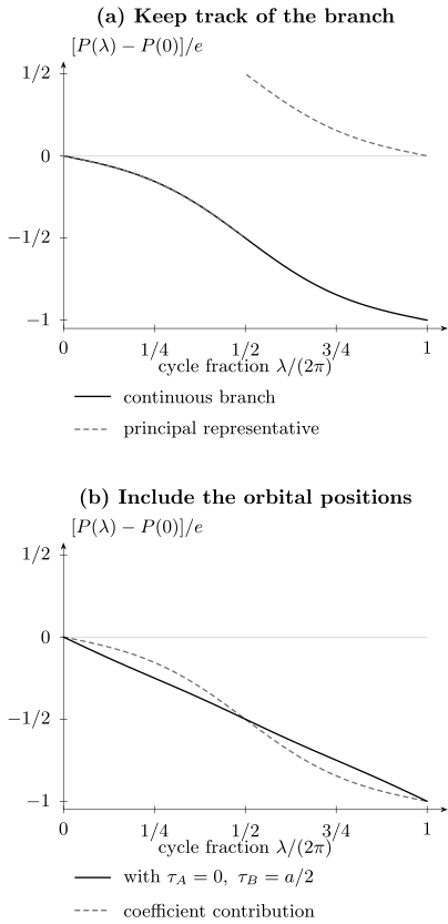
Calculated polarization changes for the stated Rice–Mele cycle. The upper panel shows the coefficient result on a continuous branch and reduced modulo $e$. The lower panel adds point-orbital positions $\tau_A=0$ and $\tau_B=a/2$. Both continuous curves change by $-e$, although their intermediate values differ. A jump of the principal representative is a branch change, not a sudden burst of transported charge.

For these orbital positions, the mean occupied weight on orbital B is

$$\bar w_B=\frac a{2\pi}\int_{\rm BZ}|c_B(k,\lambda)|^2\,dk.$$

Including this within-cell contribution gives

$$\frac{P_{\rm el}}e =\frac{\operatorname{Arg}\mathcal W_{\rm coeff}}{2\pi} -\frac{\bar w_B}{2}\pmod1.$$

Unwrap the first term before following the curve. The second term is continuous and periodic in $\lambda$, so it changes the within-cycle current but not the total transported charge. The figure uses 1200 equally spaced momenta and 241 cycle points. The ions are fixed, so they add only a constant.

One useful convergence comparison uses a uniform $N\times N$ periodic mesh, analytic derivatives of $\mathbf d$, and the rectangular quadrature rule:

$N$	Curvature integral $C$	Smallest forward $k$ overlap
12	$-1.0485272$	$0.82776$
24	$-1.0005320$	$0.93711$
48	$-1.00000005$	$0.98180$

The determinant-plaquette algorithm gives $-1$ on all three meshes, but this integer alone would conceal the coarse curvature sampling. The largest plaquette phase falls from $0.284$ to $0.0247$ radians. Gap checks, overlap conditioning, mesh refinement and comparison with the Wilson winding provide different checks of the same result. A nearly singular overlap cannot be repaired by arbitrarily assigning its phase.

A polarization change in a ferroelectric

Suppose an insulating path at fixed cell geometry starts at $P=0$ and ends with representatives $P_{\rm ion}=0.46$ and $P_{\rm el}=-0.73$, in $\mathrm{C\,m^{-2}}$. Let the polarization quantum be $0.80\ \mathrm{C\,m^{-2}}$. The endpoint sum is $-0.27$, but sufficiently close intermediate structures trace a continuous branch toward $+0.53$. The physical change along that path is therefore

$$\begin{aligned} \Delta P&=(-0.27+0.80)\ \mathrm{C\,m^{-2}}\\ &=0.53\ \mathrm{C\,m^{-2}}. \end{aligned}$$

Endpoint values alone cannot select this branch. A centrosymmetric reference also need not have the zero class: inversion permits a half-quantum class. Choose the reference from its actual charge distribution and follow the path.

For a uniform switched area $A$, the ideal electrode charge is $A\Delta P$. A real current trace includes leakage, linear capacitive charging and electrode response. Domain motion can itself contribute to polarization switching; it should not automatically be subtracted as a nonpolarization background. An incompletely switched area measures a weighted polarization change. Two-Dimensional Magnets and Ferroelectrics discusses the material-dependent interpretation.

Exercises

1. Origin shifts and a large gauge transformation

For $P=e(\tau-\bar x)/a$, shift the origin by $x_0$. Then transform an occupied Bloch state as $|u_k\rangle\mapsto e^{-ikma}|u_k\rangle$, with integer $m$. Compare the two changes.

Solution

Both positions change by $-x_0$, so their difference and the neutral total remain unchanged. The phase transformation instead gives

$$\begin{aligned} \mathcal A'_k&=\mathcal A_k+ma,\\ \gamma'&=\gamma+2\pi m,\\ P'_{\rm el}&=P_{\rm el}-me. \end{aligned}$$

This translates the chosen Wannier representative by $ma$ without changing the periodic electronic state. The bulk polarization class stays the same.

2. Recover a continuous branch

A correctly sewn rank-two forward Wilson loop has successive principal determinant phases $0,-0.60\pi,+0.80\pi,+0.40\pi,0$. Assume path refinement confirms increments smaller than $\pi$. Find the electronic polarization change for fixed orbital embedding and ions.

Solution

The continuous determinant phases are

$$0,\ -0.60\pi,\ -1.20\pi,\ -1.60\pi,\ -2\pi.$$

Since $P_{\rm el}/e=\operatorname{Arg}\det\mathcal W/(2\pi)$, the corresponding representatives are $0,-0.30,-0.60,-0.80,-1.00$. Thus $\Delta P_{\rm el}=-e$ and $C_{k\lambda}=-1$. Without sufficiently close path samples, these phases would not determine a unique winding. Without reciprocal sewing, the product would not be a closed holonomy and even its phase could depend on the endpoint frames.

3. An atomic band with a nonzero dipole

One occupied point orbital sits at $\tau=a/3$. In the cell-index Fourier convention its coefficient is $c(k)=1$. A positive ion sits at the origin. Find the total polarization class. What would a coefficient-only overlap miss?

Solution

The coefficient connection vanishes, but the orbital connection is $a/3$. Consequently $\gamma=2\pi/3$ and $P=-e/3\pmod e$. A coefficient-only calculation would give zero and lose the within-cell electronic dipole. Translating both ion and orbital by the same amount does not change the neutral total. Changing coordinates consistently is different from physically moving the electron relative to the ion.

4. What does an interface charge determine?

Two insulating regions have $P_1=0.10e$ and $P_2=0.60e$ in one dimension. The interface normal points from 1 to 2. Find the bound charge class and explain whether a measured zero net charge contradicts it.

Solution

$Q_{\rm b}=P_1-P_2=-0.50e\pmod e$. The integer part depends on termination and interface occupation. Mobile screening charge can compensate the bound charge, so zero measured net charge does not by itself contradict the bulk polarization difference. One must distinguish bound charge from total charge.

5. Pumping on a finite ring and an open chain

A finite ring has a unique gapped ground state throughout its twist–cycle torus. Does one fixed-twist current trace necessarily integrate to $eC$? Can the same conclusion be obtained by following a unique finite open-chain ground state around the cycle?

Solution

The ring theorem quantizes the twist-averaged geometric contribution. A fixed-twist value can have finite-size corrections and an equilibrium persistent-current contribution. Subtract the latter and study size and twist dependence before comparing a single trace with the integer.

A nontrivial open pump has edge spectral flow or very small edge avoided crossings. A unique finite-system state followed fully adiabatically can return to itself with no accumulated boundary charge. A pumping experiment must specify reservoirs, edge occupations or passage diabatic with respect to the tiny edge splitting while remaining adiabatic for bulk excitations. Bulk adiabaticity and complete finite-chain adiabaticity are different limits.

References

• M. V. Berry, “Quantal Phase Factors Accompanying Adiabatic Changes,” Proceedings of the Royal Society of London A 392, 45–57 (1984), doi:10.1098/rspa.1984.0023.
• R. D. King-Smith and D. Vanderbilt, “Theory of Polarization of Crystalline Solids,” Physical Review B 47, 1651–1654 (1993), doi:10.1103/PhysRevB.47.1651.
• Q. Niu and D. J. Thouless, “Quantised Adiabatic Charge Transport in the Presence of Substrate Disorder and Many-Body Interaction,” Journal of Physics A 17, 2453–2462 (1984), doi:10.1088/0305-4470/17/12/016.
• G. Ortiz and R. M. Martin, “Macroscopic Polarization as a Geometric Quantum Phase: Many-Body Formulation,” Physical Review B 49, 14202–14210 (1994), doi:10.1103/PhysRevB.49.14202.
• R. Resta, “Macroscopic Polarization in Crystalline Dielectrics: The Geometric Phase Approach,” Reviews of Modern Physics 66, 899–915 (1994), doi:10.1103/RevModPhys.66.899.
• R. Resta, “Quantum-Mechanical Position Operator in Extended Systems,” Physical Review Letters 80, 1800–1803 (1998), doi:10.1103/PhysRevLett.80.1800.
• M. J. Rice and E. J. Mele, “Elementary Excitations of a Linearly Conjugated Diatomic Polymer,” Physical Review Letters 49, 1455–1458 (1982), doi:10.1103/PhysRevLett.49.1455.
• D. J. Thouless, “Quantization of Particle Transport,” Physical Review B 27, 6083–6087 (1983), doi:10.1103/PhysRevB.27.6083.
• D. Vanderbilt, Berry Phases in Electronic Structure Theory, Cambridge University Press (2018), doi:10.1017/9781316662205.
• D. Vanderbilt and R. D. King-Smith, “Electric Polarization as a Bulk Quantity and Its Relation to Surface Charge,” Physical Review B 48, 4442–4455 (1993), doi:10.1103/PhysRevB.48.4442.
• H. Watanabe and M. Oshikawa, “Inequivalent Berry Phases for the Bulk Polarization,” Physical Review X 8, 021065 (2018), doi:10.1103/PhysRevX.8.021065.
• D. Xiao, M.-C. Chang, and Q. Niu, “Berry Phase Effects on Electronic Properties,” Reviews of Modern Physics 82, 1959–2007 (2010), doi:10.1103/RevModPhys.82.1959.
• J. Zak, “Berry’s Phase for Energy Bands in Solids,” Physical Review Letters 62, 2747–2750 (1989), doi:10.1103/PhysRevLett.62.2747.