Boundary Conditions on Lattices

A boundary condition on a finite lattice specifies how the finite set of sites, links, and local operators closes. On a chain, an open boundary omits the bond between the last and first sites, a periodic boundary adds that wrapping bond, and a twisted boundary adds it with a phase or internal-symmetry rotation. This apparently small choice changes exact symmetries, momentum labels, edge degrees of freedom, finite-size spectra, and sometimes the algebraic form of an exact solution.

Boundary conditions are part of the Hamiltonian, not a numerical option applied after the model is defined. Two calculations using the same local bulk term but different closures are different finite systems. They may approach the same thermodynamic bulk phase while retaining sharply different edge and finite-size physics.

Helpful background. Tight-binding modes supplies the one-particle spectra; translations explains momentum labels.

Sites, bonds and wrapping terms

A lattice model begins with a graph $G=(V,E)$:

• vertices $V$ carry local Hilbert spaces or orbitals;
• edges $E$ specify which pairs are coupled;
• oriented edges may carry complex hopping or exchange phases;
• plaquettes and noncontractible loops carry gauge-invariant phase products.

For a nearest-neighbor chain with sites $j=1,\ldots,L$, write a generic local Hamiltonian as

$$H = \sum_{j=1}^{L}h_j + \sum_{(j,k)\in E}h_{jk}.$$

The open and periodic edge sets are

$$E_{\mathrm O} = \{(1,2),(2,3),\ldots,(L-1,L)\},$$ $$E_{\mathrm P} = E_{\mathrm O}\cup\{(L,1)\}.$$

Thus an open nearest-neighbor chain has $L-1$ bonds, whereas a periodic ring has $L$ bonds. The difference is one local term, but that term changes the graph topology from an interval to a cycle.

Write the wrapping term explicitly

For finite calculations, the safest convention is to write the wrapping term before replacing indices modulo $L$. This exposes:

• its phase and orientation;
• whether it is counted once or twice;
• whether it preserves the intended symmetry;
• whether a nonlocal transformation inserts a parity operator;
• whether a very short ring creates repeated or self-couplings.

Only after these checks should one use shorthand such as $j+L\equiv j$.

Short-system caveat

Modulo indexing can silently double count bonds. A nearest-neighbor cycle graph with $L\ge3$ has $L$ undirected edges. For $L=2$, the formal terms $j=1$ and $j=2$ can both describe the same undirected pair. Whether they represent one bond, two parallel directed bonds, or a doubled coupling depends on the model convention. Small-system benchmarks must use the same graph definition as the analytic formula.

Open Boundaries

An open chain contains no wrapping interaction. For nearest-neighbor terms,

$$H_{\mathrm O} = \sum_{j=1}^{L}h_j + \sum_{j=1}^{L-1}h_{j,j+1}.$$

Open boundaries create physical edge sites with reduced coordination. They generally:

• break translation symmetry;
• preserve a midpoint reflection when the couplings are symmetric;
• permit boundary-localized or topological edge states;
• allow a single domain wall to terminate at an edge;
• add surface contributions to energies and observables;
• make matrix-product-state calculations substantially cheaper than periodic geometry.

Open does not mean deleting the endpoint sites

For a one-particle nearest-neighbor recurrence, it is convenient to introduce fictitious amplitudes

$$\psi_0=0, \qquad \psi_{L+1}=0.$$

These encode the absence of hopping beyond sites $1$ and $L$. The physical amplitudes $\psi_1$ and $\psi_L$ need not vanish. Confusing the fictitious nodes with the actual edge sites removes legitimate boundary weight and can erase edge states.

For a uniform open hopping chain, the standing-wave labels are

$$q_m = \frac{\pi m}{L+1}, \qquad m=1,\ldots,L.$$

The eigenfunctions are proportional to $\sin(q_mj)$. Since one-site translation is not an exact symmetry, $q_m$ is a standing-wave label rather than a conserved crystal momentum.

Boundary terms are allowed

Open geometry does not require the edge Hamiltonian to equal a truncated bulk term. One may add

$$H_{\mathrm{edge}} = v_1+v_L+h_{1,\mathrm{aux}}+h_{L,\mathrm{aux}},$$

where $v_1,v_L$ are local edge potentials and auxiliary couplings attach leads, impurity spins, reservoirs, or boundary fields. These terms define a new boundary condition or boundary universality class; they should not be hidden inside the phrase open boundary conditions.

Periodic Boundaries

A periodic chain closes the last site onto the first:

$$H_{\mathrm P} = \sum_{j=1}^{L}h_j + \sum_{j=1}^{L}h_{j,j+1}, \qquad h_{L,L+1}\equiv h_{L,1}.$$

For uniform couplings, translation by one site is an exact symmetry. Let $T$ be the unitary translation operator with

$$T^L=I, \qquad [H_{\mathrm P},T]=0.$$

Its eigenvalues are roots of unity,

$$T|K,\alpha\rangle = e^{iK}|K,\alpha\rangle,$$ $$K = \frac{2\pi m}{L} \pmod{2\pi}, \qquad m=0,\ldots,L-1.$$

Here $K$ is dimensionless many-body lattice momentum. With spacing $a$, the corresponding wave number is $k=K/a$. To fix the sign, choose $Tc_j^\dagger T^{-1}=c_{j-1}^\dagger$ (indices modulo $L$) and $T|\mathrm{vac}\rangle=|\mathrm{vac}\rangle$. Then a mode created by $L^{-1/2}\sum_j e^{ikja}c_j^\dagger$ has translation eigenvalue $e^{ika}$.

Periodic is not open with distant edges coupled weakly

The bond $(L,1)$ is a nearest-neighbor bond in the cycle graph. It has the same locality status as $(j,j+1)$ even if a drawing places sites $L$ and $1$ far apart. Conversely, adding a small coupling between physical ends of an open sample is a boundary perturbation, not automatically periodic geometry unless it completes the intended translation-invariant cycle.

No physical edge

A periodic ring has no boundary vertices. It cannot host an edge state that requires a termination, although it may have defects, domain walls, fluxes, or topological sectors. Comparing open and periodic spectra is therefore a direct way to distinguish bulk states from boundary-localized states.

Twisted and Antiperiodic Boundaries

Suppose the model has a conserved $U(1)$ charge and an annihilation operator $c_j$ carrying one unit of that charge. A spatial twist $\phi$ imposes

$$c_{j+L} = e^{i\phi}c_j,$$ $$c_{j+L}^\dagger = e^{-i\phi}c_j^\dagger.$$

Important cases are

$$\phi=0 \quad\text{periodic},$$ $$\phi=\pi \quad\text{antiperiodic}.$$

The phase is defined modulo $2\pi$.

Boundary-link gauge

For real nearest-neighbor hopping in the interior, place the whole twist on the wrapping bond:

$$H(\phi) ={} -t\sum_{j=1}^{L-1} (c_j^\dagger c_{j+1}+c_{j+1}^\dagger c_j) - t\left( e^{i\phi}c_L^\dagger c_1 + e^{-i\phi}c_1^\dagger c_L \right).$$

Hermiticity requires the reverse hopping to carry the conjugate phase. Reversing the chosen orientation sends $\phi\to-\phi$.

Uniform-link gauge

The site-dependent rephasing

$$c_j = e^{ij\phi/L}d_j$$

makes $d_{j+L}=d_j$ and distributes the phase uniformly:

$$H(\phi) = -t\sum_{j=1}^{L} \left( e^{i\phi/L}d_j^\dagger d_{j+1} + e^{-i\phi/L}d_{j+1}^\dagger d_j \right).$$

The phase on a particular link is gauge dependent. The total holonomy around the ring,

$$\prod_{j=1}^{L}e^{i\phi/L} = e^{i\phi},$$

is invariant under single-valued site rephasings.

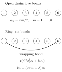
The same six sites have five bonds when open and six when closed into a ring. A real wrapping term gives the periodic model; conjugate phases on that term give a twisted ring. The arc represents a nearest-neighbor bond of the ring graph, regardless of its length in the drawing.

Momentum grid

A plane wave $c_j\sim e^{ikja}$ obeys the twist when

$$e^{ikLa} = e^{i\phi}.$$

Therefore

$$k_m(\phi) = \frac{2\pi m+\phi}{La}.$$

The twist shifts the sampled momenta through the same translation-invariant bulk dispersion. It does not generally change the continuous band function itself.

The unordered spectrum is $2\pi$ periodic:

$$\operatorname{Spec}H(\phi+2\pi) = \operatorname{Spec}H(\phi).$$

Individual eigenvalue branches can permute as $\phi$ advances by $2\pi$. This spectral flow contains physical information and should not be erased by relabeling too early.

Flux interpretation

For charge $q$ moving around a ring threaded by vector potential $\mathbf A$, the twist is the Aharonov–Bohm holonomy

$$\phi = \frac{q}{\hbar} \oint\mathbf A\cdot d\boldsymbol\ell \pmod{2\pi},$$

with sign fixed by charge and path orientation. A gauge transformation can move the vector potential into a boundary phase, but it cannot remove a nontrivial loop holonomy. Peierls Phase Preview develops the lattice gauge principle and plaquette fluxes.

Twists for spins

For a spin chain with conserved total $S^z$, a $U(1)$ spin twist can be defined by

$$s_{L+1}^{\pm} = e^{\pm i\phi}s_1^{\pm}, \qquad s_{L+1}^{z}=s_1^z.$$

The transverse exchange on the wrapping bond acquires conjugate phases while the longitudinal exchange does not. This probes spin stiffness rather than electric charge response.

Species-dependent twists

For spinful particles or several components, one may choose phases $\phi_\sigma$. Equal twists probe total charge motion. Opposite twists can probe spin or counterflow response. A calculation must state which conserved generator the twist couples to; the phrase twisted boundary conditions alone is incomplete.

Mode Grids at a Glance

For a uniform nearest-neighbor chain of $L$ sites, the common one-particle labels are:

Boundary	Identification or endpoint rule	Mode label	Exact translation sector?
open	no $(L,1)$ bond; fictitious $\psi_0=\psi_{L+1}=0$	$q_m=\pi m/(L+1)$, $m=1,\ldots,L$	no
periodic	$c_{j+L}=c_j$	$k_m=2\pi m/(La)$	yes
antiperiodic	$c_{j+L}=-c_j$	$k_m=(2m+1)\pi/(La)$	twisted translation
twisted	$c_{j+L}=e^{i\phi}c_j$	$k_m=(2\pi m+\phi)/(La)$	twisted translation

Every row contains exactly $L$ one-particle modes. Different integer ranges merely choose different representatives modulo the reciprocal-lattice period $2\pi/a$.

Do not mix denominators

The $L+1$ in the open standing-wave grid comes from the two fictitious nodes outside the physical chain. The $L$ in the periodic grid comes from winding around $L$ lattice spacings. Substituting one denominator for the other changes the finite Hamiltonian.

Momentum modulo a reciprocal vector

On a lattice,

$$k \sim k+\frac{2\pi}{a}.$$

A finite ring selects $L$ representatives from this equivalence class. The Brillouin-zone endpoint must not be counted twice.

Many-Body Momentum Sectors

For a periodic translation-invariant Hamiltonian, $T$ commutes with particle number, spin components preserved by the model, and the Hamiltonian. The Hilbert space decomposes as

$$\mathcal H = \bigoplus_K\mathcal H_K.$$

Exact diagonalization can work independently in each $K$ sector. This reduces matrix size and prevents unrelated symmetry blocks from contaminating level statistics.

Translation orbits of basis states

Let $|s\rangle$ be a product or occupation basis state, and let $r$ be the shortest period of its occupation pattern. A spin product basis has $T^r|s\rangle=|s\rangle$, but a fermion occupation basis can acquire a reordering sign:

$$T^r|s\rangle=\eta_s|s\rangle,\qquad \eta_s=\pm1.$$

A momentum-adapted vector is

$$|s;K\rangle=\frac1{\sqrt r}\sum_{n=0}^{r-1}e^{-iKn}T^n|s\rangle, \qquad e^{iKr}=\eta_s.$$

The compatibility condition follows by translating the last term back to the first. Omitting the fermionic sign can put states in the wrong momentum sector. For example, translating the four-site fermion pattern $1010$ by two sites exchanges its two creation operators: $\eta_s=-1$. Its two orbit states contribute to $K=\pm\pi/2$, whereas the same spin pattern contributes to $K=0,\pi$.

Total momentum for free modes

For independent periodic modes,

$$K_{\mathrm{tot}} = a\sum_k k n_k \pmod{2\pi}.$$

Interactions can mix occupation configurations while preserving their total $K_{\mathrm{tot}}$. Momentum conservation does not imply that individual particle momenta remain good quantum numbers.

Twisted translation

In a boundary-link gauge, ordinary translation moves the distinguished phased bond and may not visibly commute with the Hamiltonian. In a uniform-link gauge, all bonds carry the same phase and one-site translation is manifest. The two descriptions are unitarily equivalent; symmetry cannot depend on where a gauge places the phase.

For many particles, translating every particle around a twisted ring can accumulate a charge-dependent phase. State the translation operator and gauge convention before assigning momentum labels.

Open chains use other symmetries

An open uniform chain has no cyclic momentum sectors. It may have reflection parity,

$$R^2=I, \qquad [H_{\mathrm O},R]=0,$$

as well as internal symmetries such as particle number or total spin. Labeling an open-chain standing wave by $q_m$ is useful, but calling it an exact many-body momentum sector is misleading.

Fermion-Parity Caveat

Spatial periodicity for microscopic fermions and effective periodicity after a nonlocal spin transformation are different constructions.

Directly defined fermion ring

If the microscopic degrees of freedom are fermions on a ring, periodic, antiperiodic, or twisted spatial boundary conditions are independent model choices:

$$c_{L+1}=e^{i\phi}c_1.$$

No extra parity rule appears merely because the particles are fermions.

Fermions obtained from a periodic spin chain

For the Jordan–Wigner convention used in this volume, a periodic spin chain gives

$$c_{L+1} = -p c_1, \qquad p=(-1)^N.$$

Thus

Fermion parity $p$	Effective spatial fermion boundary	Mode grid
$+1$	antiperiodic	$k=(2m+1)\pi/(La)$
$-1$	periodic	$k=2\pi m/(La)$

The workflow is:

1. select a parity sector $p$;
2. impose the matching fermion boundary condition;
3. diagonalize the sector Hamiltonian;
4. retain only many-body states with physical parity $p$.

The boundary sign follows from the Jordan–Wigner string crossing the ordering cut. Jordan–Wigner Transformation gives the operator proof and treats the self-inverse $k=0$ and $k=\pi/a$ modes.

Pairing does not remove parity

A Bogoliubov Hamiltonian can violate particle-number conservation while preserving fermion parity. Its periodic and antiperiodic sectors must still be matched to the original spin sector. Diagonalizing both grids and keeping every quasiparticle state generally doubles the physical Hilbert space. The quasiparticle vacuum may itself have odd original-fermion parity, so enforce $P=p_{\mathrm{vac}}(-1)^{N_\gamma}$ rather than assuming $P=(-1)^{N_\gamma}$.

Spatial versus imaginary-time antiperiodicity

Spatial antiperiodic boundary conditions are a choice of finite geometry or flux. Fermionic fields in the ordinary full-Fock-space thermal trace are antiperiodic around the Euclidean-time circle. Fixed-number projection adds a number-selecting phase integral, and fixed-parity projection combines different temporal trace sectors; those projected ensembles require their own prescription. These are different cycles and different statements. One does not imply the other.

Boundary Counting in Higher Dimensions

Consider a $d$-dimensional hyperrectangle with $L_\mu$ sites along direction $\mu$ and

$$V = \prod_{\mu=1}^{d}L_\mu$$

total sites. With open boundaries in every direction, the number of nearest-neighbor undirected bonds is

$$B_{\mathrm O} = \sum_{\mu=1}^{d} (L_\mu-1) \prod_{\nu\ne\mu}L_\nu.$$

With periodic boundaries in every direction and nondegenerate lengths,

$$B_{\mathrm P} = dV.$$

The missing-bond fraction scales like surface area divided by volume. For an isotropic $L^d$ sample,

$$\frac{B_{\mathrm P}-B_{\mathrm O}}{V} = \frac{d}{L}.$$

The formula assumes each periodic direction defines an ordinary cycle rather than a short multigraph. Very small $L_\mu$ again requires explicit edge counting.

Cylinder, torus, and slab

Boundary conditions may differ by direction:

• periodic in every direction gives a torus;
• periodic along one direction and open along another gives a cylinder;
• periodic in-plane and open transversely gives a slab;
• open in every direction gives a finite cluster with corners.

These geometries separate bulk, edge, hinge, and corner responses. A page or data file should list the choice in every primitive direction, not merely say mixed boundaries.

Twist vector

On a $d$-dimensional torus, assign a twist vector

$$\boldsymbol\phi = (\phi_1,\ldots,\phi_d).$$

The single-particle grid becomes

$$k_\mu = \frac{2\pi m_\mu+\phi_\mu}{L_\mu a_\mu}.$$

Each $\phi_\mu$ is a holonomy around a noncontractible cycle. It is distinct from the flux through an elementary plaquette, although both are represented by products of link phases.

Periodic images and long-range interactions

For short-range Hamiltonians, wrapping local bonds defines periodicity. For Coulomb, dipolar, or other long-range interactions, one must also specify how periodic images are summed. Minimum-image truncation, Ewald summation, and a direct finite-cluster interaction define different finite Hamiltonians. The words periodic boundary conditions do not settle this choice.

Bulk and Boundary Energy Scaling

For a one-dimensional local Hamiltonian with a well-defined bulk energy density $e_\infty$, typical large-$L$ forms are

$$E_{\mathrm O}(L) = Le_\infty +e_{\mathrm s} +\delta E_{\mathrm O}(L),$$ $$E_{\mathrm P}(L) = Le_\infty +\delta E_{\mathrm P}(L).$$

The open chain has an $O(1)$ surface energy $e_{\mathrm s}$. Dividing by $L$ makes this a $1/L$ correction to the energy density. The periodic chain has no physical surface term, but it still has finite-size corrections from quantized modes, virtual winding processes, and sector constraints.

Gapped systems

When a periodic system has a unique gapped bulk ground state and correlation length $\xi$, many local finite-size corrections are exponentially small,

$$\delta E_{\mathrm P}(L) \sim e^{-La/\xi},$$

up to prefactors and exceptions associated with topology, conserved sectors, or nearly degenerate vacua. Open systems can have $O(1)$ edge energies and exponentially small splittings between edge degrees of freedom.

Critical systems

A finite critical chain has a nonzero level spacing even though the thermodynamic gap vanishes. Here $L$ counts sites, $a$ is the spacing and $\xi$ is a physical length. For a relativistic critical point with physical velocity $v$, the characteristic scale is

$$\Delta E(L) \sim \frac{\hbar v}{La}.$$

In conformal cases, periodic levels often have the form

$$E_n(L)-E_0(L) = \frac{2\pi\hbar v}{La}x_n +o(L^{-1}),$$

whereas open boundaries organize boundary scaling dimensions with a characteristic factor $\pi\hbar v/(La)$. The allowed $x_n$, degeneracies, and additive terms depend on the boundary and symmetry sector. A finite gap at one $L$ is therefore not evidence for a gapped phase.

Compare like with like

When comparing open and periodic total energies, first account for:

• the different number of bonds;
• surface fields or edge potentials;
• different allowed symmetry sectors;
• distinct shell fillings;
• whether the observable is total, per site, or per bond.

Bulk extrapolation should use intensive quantities and several sizes. Edge physics should be studied through boundary-local observables rather than divided away.

Shell Effects and Degeneracies

A finite periodic system samples a continuous dispersion at a discrete grid. Whether a sampled momentum lands exactly on a band crossing or Fermi point can change:

• ground-state degeneracy;
• the particle number of a closed shell;
• the apparent excitation gap;
• persistent current and stiffness estimates;
• which momentum sector contains the ground state.

Periodic and antiperiodic grids interlace. Comparing both is often more informative than treating either as uniquely correct for a bulk extrapolation.

Odd–even effects

Odd and even lengths can realize different graph properties. An even nearest-neighbor ring is bipartite; an odd ring is not. An antiferromagnetic Ising ring of odd length cannot fit a perfectly alternating pattern. For Heisenberg spins, odd cycles also frustrate collinear Néel order, though even quantum chains already cannot minimize every bond independently as a singlet.

Likewise, an untwisted periodic Ising ring has an even number of sign changes $z_j\ne z_{j+1}$, while an open chain can contain a single wall. Such constraints can move the lowest state between sectors and change the first finite-size gap without changing the local bulk Hamiltonian.

Commensurability

Charge-density waves, spin spirals, and enlarged unit cells fit cleanly only when the finite dimensions are commensurate with their ordering wave vectors. An incompatible periodic cluster can force a defect or suppress an order parameter. Checking several cluster shapes is essential before concluding that an ordered phase is absent.

Flux Response and Stiffness

The dependence of the ground-state energy on a twist probes coherent transport around a ring. If physical flux $\Phi$ produces twist $\phi(\Phi)$, the persistent current is

$$I(\Phi) = -\frac{\partial E_0}{\partial\Phi}.$$

A charge or spin stiffness is proportional to the curvature

$$\mathcal D_L \propto L^{2-d} \left. \frac{\partial^2E_0} {\partial\phi^2} \right|_{\phi=0},$$

for an isotropic $d$-dimensional sample of linear site count $L$, if the selected ground-energy branch is smooth at zero twist. At a crossing, a second derivative may not exist; a smooth branch or a specified minimizing twist must be used instead. The displayed quantity has energy units before restoring geometric or charge factors. Rectangular samples require the corresponding length and volume factors.

An insulator is typically insensitive to a distant boundary twist in the thermodynamic limit, whereas a superfluid or a clean ballistic metal can retain finite stiffness. A generic conductor need not have a nonzero Drude weight: diffusive dc transport and a delta-function zero-frequency response are different notions. Finite-size level crossings, degeneracies, disorder averaging, and order of limits can complicate this diagnostic.

Twist averaging

Finite momentum-shell errors can be reduced by averaging an observable over twists:

$$\overline{O} = \frac{1}{(2\pi)^d} \int_0^{2\pi}d^d\phi\, O(\boldsymbol\phi).$$

In practice the integral is sampled on a finite twist grid. Twist averaging improves one-body momentum sampling and can smooth shell effects. It does not eliminate interaction finite-size errors, topological sector changes, or the need for size extrapolation.

Edges, Topology, and Entanglement

Open and periodic geometries answer different physical questions.

Edge states

A state localized near a termination can exist only when the relevant boundary is present. Its energy may lie in a bulk gap, and two opposite-edge modes can hybridize with a splitting

$$\Delta E_{\mathrm{edge}} \sim e^{-La/\xi_{\mathrm{edge}}}.$$

Closing the chain removes those physical edges. If the in-gap states disappear while the bulk bands remain, that is evidence for boundary localization, not a change in the bulk Hamiltonian.

Entanglement geometry

A proper interval on a ring has two entanglement cuts. An interval attached to the end of an open chain has one, but an interval wholly inside the open chain still has two. At a one-dimensional conformal critical point, this changes the logarithmic coefficient and boundary constants. The canonical entropy definitions and scaling caveats are on Entanglement Entropy in Many-Body Systems.

Bulk topology from twists

Periodic twists can probe bulk topology without introducing edges. A one-dimensional twist cycle can define a many-body polarization phase. Two independent twist angles can define a many-body Chern number under suitable smoothness, gap and nondegeneracy assumptions. This is distinct from merely observing an edge state; bulk and boundary diagnostics should cross-check one another.

Exercises

Count bonds on a rectangle

A square-lattice cluster has $L_x=4$ and $L_y=5$. Count nearest-neighbor undirected bonds for:

1. open boundaries in both directions;
2. periodic $x$ and open $y$ boundaries;
3. periodic boundaries in both directions.

Assume the dimensions are large enough that no short-cycle duplicate arises.

Solution

There are $V=L_xL_y=20$ sites. With both directions open,

$$B_{\mathrm{OO}} = (L_x-1)L_y + (L_y-1)L_x.$$

Therefore

$$B_{\mathrm{OO}} = 3\cdot5+4\cdot4 = 31.$$

Making $x$ periodic adds one wrapping $x$ bond in each of the five rows:

$$B_{\mathrm{PO}} = L_xL_y + (L_y-1)L_x = 20+16 = 36.$$

On the torus, each site contributes one positively oriented bond in each of two directions:

$$B_{\mathrm{PP}} = 2V = 40.$$

Counting only positive directions avoids counting each undirected bond twice.

Translation signs of a fermion pattern

On a six-site periodic chain, take the ordered fermion state $|s\rangle=|100100\rangle$. Find its pattern period and compatible momenta, including creation-operator signs. Compare with the corresponding spin product state.

Solution

The pattern returns after three translations. But this exchanges the two occupied fermionic modes, so $T^3|s\rangle=-|s\rangle$. Hence

$$e^{3iK}=-1,\qquad K\in\{\pi/3,\pi,5\pi/3\}.$$

They are the $m=1,3,5$ sectors of $K=2\pi m/6$. For spin product states there is no fermionic reordering sign, so $\eta_s=+1$ and the corresponding momenta are $0,2\pi/3,4\pi/3$. The pattern period alone does not determine the answer.

Spectral flow under a full twist

For a free nearest-neighbor ring,

$$\varepsilon_m(\phi) = -2t\cos \left( \frac{2\pi m+\phi}{L} \right),$$

show that increasing $\phi$ by $2\pi$ leaves the spectrum invariant as a set. Does each fixed-$m$ branch return to itself?

Solution

Evaluate

$$\varepsilon_m(\phi+2\pi) = -2t\cos \left( \frac{2\pi(m+1)+\phi}{L} \right).$$

Therefore

$$\varepsilon_m(\phi+2\pi) = \varepsilon_{m+1}(\phi).$$

The set of $L$ energies is unchanged because $m$ is defined modulo $L$. A branch followed with fixed label $m$ flows into its neighbor rather than necessarily returning to itself after one flux quantum. After $L$ such cycles the simple fixed-label branch returns.

Frustration on an odd ring

Let classical Ising variables $z_j=\pm1$ have antiferromagnetic energy

$$E = J\sum_{\langle j,k\rangle}z_jz_k, \qquad J>0.$$

Find the minimum energy for an open chain and for an odd periodic ring. Count the ground states of the odd ring.

Solution

An antialigned bond contributes $-J$. On an open chain, all $L-1$ bonds can be antialigned:

$$E_{\mathrm O}^{\min} = -(L-1)J.$$

On an odd ring, alternating signs cannot close consistently. At least one of the $L$ bonds must be aligned. A minimum configuration has $L-1$ satisfied bonds and one frustrated bond, so

$$E_{\mathrm P}^{\min} = -(L-1)J+J = -(L-2)J.$$

The frustrated bond can occupy any of the $L$ positions, and a global spin flip gives a distinct configuration. The ground-state degeneracy is therefore

$$2L.$$

The extensive bulk energy density still approaches $-J$, but the odd periodic topology enforces an $O(1)$ defect.

References

• N. Byers and C. N. Yang, “Theoretical Considerations Concerning Quantized Magnetic Flux in Superconducting Cylinders”, Physical Review Letters 7, 46–49 (1961).
• M. E. Fisher and M. N. Barber, “Scaling Theory for Finite-Size Effects in the Critical Region”, Physical Review Letters 28, 1516–1519 (1972).
• W. Kohn, “Theory of the Insulating State”, Physical Review 133, A171–A181 (1964).
• E. Lieb, T. Schultz, and D. Mattis, “Two Soluble Models of an Antiferromagnetic Chain”, Annals of Physics 16, 407–466 (1961).
• C. Lin, F. H. Zong, and D. M. Ceperley, “Twist-Averaged Boundary Conditions in Continuum Quantum Monte Carlo Algorithms”, Physical Review E 64, 016702 (2001).
• Q. Niu, D. J. Thouless, and Y.-S. Wu, “Quantized Hall Conductance as a Topological Invariant”, Physical Review B 31, 3372–3377 (1985).
• M. Oshikawa, “Commensurability, Excitation Gap, and Topology in Quantum Many-Particle Systems on a Periodic Lattice”, Physical Review Letters 84, 1535–1538 (2000).
• R. Resta, “Quantum-Mechanical Position Operator in Extended Systems”, Physical Review Letters 80, 1800–1803 (1998).
• B. S. Shastry and B. Sutherland, “Twisted Boundary Conditions and Effective Mass in Heisenberg–Ising and Hubbard Rings”, Physical Review Letters 65, 243–246 (1990).
• S. R. White, “Density Matrix Formulation for Quantum Renormalization Groups”, Physical Review Letters 69, 2863–2866 (1992).