Wannierization Workflows

Wannierization constructs localized orbitals from Bloch states. These orbitals can turn a large band calculation into a compact Hamiltonian that is cheap to evaluate at new momenta. The central practical question is what the compact representation preserves. Reproducing a band plot does not by itself ensure that the retained states, spin matrix elements, or optical response are accurate. This guide separates subspace selection, localization, interpolation, and tests of the resulting operators, including a small exact model.

Required background. Wannier functions introduces Bloch projectors, basis freedom, and the Bloch–Wannier transform. Band structure workflows explains how to obtain a converged source Hamiltonian and sample the full Brillouin zone.

Bloch subspaces and their bases

A subspace specifies which states are retained. A basis specifies how those states are described. Changing an orthonormal basis within one subspace changes matrices but preserves predictions when all states and operators are transformed together. Changing the subspace can change the predictions themselves.

Let the columns of $\Psi_{\mathbf k}$ be orthonormal source Bloch states, with $\Psi_{\mathbf k}^{\dagger}\Psi_{\mathbf k}=I$. Choose $J$ combinations through a rectangular matrix $V_{\mathbf k}$, then rotate their basis with $U_{\mathbf k}$:

$$V_{\mathbf k}^{\dagger}V_{\mathbf k}=I_J, \qquad U_{\mathbf k}\in U(J).$$ $$\begin{aligned} Q_{\mathbf k}&=V_{\mathbf k}U_{\mathbf k},\\ \Phi_{\mathbf k}&=\Psi_{\mathbf k}Q_{\mathbf k},\\ P_{\mathbf k}&=\Phi_{\mathbf k}\Phi_{\mathbf k}^{\dagger}. \end{aligned}$$

Here $\Phi$ is an orthonormal frame: an ordered basis varying with momentum. The projector $P$ depends on $V$ but not on $U$. A momentum-dependent $U$ can change individual orbital centers, spreads, and hoppings while leaving the represented subspace unchanged.

For an isolated band family, its spectral projector is separated from excluded bands at every momentum. Crossings within the family are allowed. One may take the source frame to contain exactly these $J$ states, so that no subspace selection is needed. Direct isolation does not require an indirect insulating gap or a completely occupied family.

For entangled bands, the desired $J$ states must instead be selected from a larger space. Changing $V$ changes the retained projector. The disentanglement method of Souza, Marzari, and Vanderbilt (2001) selects a subspace that varies smoothly across momentum, before optimizing its internal basis. Smoothness is useful, but the resulting states must still describe the physics of interest.

Choose the intended use before choosing tolerances. Energy interpolation for a density of states, spin matrix elements, and optical transitions require different comparisons. A small energy error cannot replace an operator test.

Source states and the physical inner product

Hold the source Hamiltonian fixed while studying Wannierization errors. Changing the crystal structure, density, magnetic state, functional, or relativistic treatment changes the physical calculation. Increasing the Wannier mesh or hopping range addresses a different question.

Retain the eigenvalues and states, lattice and reciprocal vectors, orbital positions, spinor conventions, neighbor overlaps, and physical matrices of the operators you will use. Eigenvalues alone contain no information about relative phases or orbital character. Keep the input parameters and software versions so another calculation can reproduce these quantities.

In a nonorthogonal coefficient basis, normalization uses its positive overlap matrix $S_{\mathbf k}$:

$$C_{\mathbf k}^{\dagger}S_{\mathbf k}C_{\mathbf k}=I.$$

Euclidean normalization of the coefficient columns generally gives the wrong inner product. Likewise, a neighbor overlap involves two different bases:

$$M(\mathbf k,\mathbf b) =C_{\mathbf k}^{\dagger} S_{\mathbf k,\mathbf k+\mathbf b} C_{\mathbf k+\mathbf b}.$$

The cross-momentum matrix includes the physical overlap and the reciprocal boundary identification when the neighbor lies outside the chosen zone. Replacing it by $S_{\mathbf k}$ is not generally valid. Boundary phases, spin rotations, and orbital positions must be consistent across all links.

If $O^{\rm phys}_{\mathbf k}$ contains physical operator matrix elements in the coefficient basis, its source-state matrix is $C_{\mathbf k}^{\dagger}O^{\rm phys}_{\mathbf k}C_{\mathbf k}$. The alternative expression $C^{\dagger}SO^{\rm coeff}C$ applies only when $O^{\rm coeff}$ is explicitly the coefficient-action matrix. Distinguishing these conventions prevents an extra or missing factor of $S$.

An isolated family needs a direct separation from its complement throughout the zone. An entangled calculation needs enough source states everywhere to support its chosen rank and mandatory states. A plotting path tests neither condition over the full zone.

Trial orbitals, windows, and frozen states

Trial orbitals provide an initial guess. First remove their linear dependencies and normalize their span in the physical inner product. For independent physical trial columns $G$, an orthonormal choice is

$$\overline G=G(G^{\dagger}G)^{-1/2}.$$

In a nonorthogonal coefficient basis replace $G^{\dagger}G$ by $G^{\dagger}SG$. Project the normalized trials into the source space:

$$\begin{aligned} A&=\Psi^{\dagger}\overline G,\\ \mathcal G&=A^{\dagger}A,\\ V^{(0)}&=A\mathcal G^{-1/2}. \end{aligned}$$

The last expression requires full column rank. For normalized frames, the singular values of $A$ measure how well the source space contains the trial directions. A small positive value means that one projected direction has a small norm and can be sensitive to perturbations; zero means rank loss. Arbitrarily rescaling an unnormalized trial changes these values without changing its span. Thus a numerical threshold needs a fixed normalization and a relevant error scale. Check conditioning throughout the mesh.

The outer window supplies available source states. The frozen window specifies source eigenstates that the selected subspace must contain exactly, up to numerical tolerance. These meanings are described in the Wannier90 parameter documentation. Necessary pointwise conditions are

$$N_{\rm out}(\mathbf k)\ge J, \qquad N_{\rm fr}(\mathbf k)\le J.$$

For an orthonormal frozen-state matrix $F$ expressed in the outer frame, test

$$r_{\rm fr}=\|(I-VV^{\dagger})F\|_2.$$

These counts alone do not guarantee a smooth or symmetry-compatible solution. An impossible state count makes the requested construction infeasible. A residual above tolerance means the computed subspace does not contain the required states; it can also reveal a convergence or implementation problem in an otherwise feasible calculation. Do not confuse these diagnoses.

Try physically plausible alternatives in windows and orbital character. For spinors, specify whether trials represent actual spin orbitals or an effective pseudospin, and include the correct local axes and site positions. Changing rank or windows changes the selected model; additional optimizer iterations alone cannot establish stability under those changes.

Localization and symmetry

Localization is controlled by the variation of the selected cell-periodic frame across momentum. Its neighbor overlaps are

$$M_{mn}^{(\mathbf k,\mathbf b)} =\langle u^{(\Phi)}_{m\mathbf k} \mid u^{(\Phi)}_{n,\mathbf k+\mathbf b}\rangle.$$

Use the boundary identification before taking the inner product. Naively wrapping stored components can create a discontinuity that is absent from the physical states.

The quadratic spread separates as $\Omega=\Omega_I+\widetilde\Omega$. At fixed projector, $\Omega_I$ is independent of the internal basis, whereas $\widetilde\Omega$ changes with it. A standard discrete expression is

$$\Omega_I=\frac1{N_k}\sum_{\mathbf k,\mathbf b}w_{\mathbf b} \left[J-\sum_{m,n}|M_{mn}^{(\mathbf k,\mathbf b)}|^2\right],$$

with finite-difference weights $w_{\mathbf b}$ appropriate to the mesh. Marzari and Vanderbilt (1997) develop the spread minimization; the review by Marzari et al. (2012) explains its relation to disentanglement. Comparing spreads across different projectors mixes subspace selection with basis optimization. The smaller spread need not give more accurate observables.

Compare several starting guesses, residuals, individual spreads, and orbital centers as the mesh is refined. If symmetry is imposed, check its action on the frame as well. For a unitary source symmetry $B_g$ and desired orbital representation $D_g$,

$$B_g(\mathbf k)Q_{\mathbf k} =Q_{g\mathbf k}D_g(\mathbf k).$$

An antiunitary action conjugates $Q_{\mathbf k}$ on the left. Include spin, fractional translations, and reciprocal boundary phases. Symmetry constraints can increase the smallest attainable spread; Sakuma (2013) describes a symmetry-adapted construction.

Failure to converge does not establish a topological obstruction. A nonzero Chern number does obstruct exponentially localized orthonormal translated Wannier functions for that isolated projector. The existence assumptions are developed in Wannier functions and Chern numbers. Requirements on a symmetry-preserving basis are additional conditions; use symmetry of Bloch states when deciding which symmetry constraints are appropriate.

Equal energies can hide different subspaces

Consider three orthonormal internal states and the one-dimensional source Hamiltonian

$$\begin{aligned} \widehat H(q)&=\epsilon(q)I +\Delta\operatorname{diag}(-1,0,1),\\ \epsilon(q)&=2t\cos q,\qquad q=ka. \end{aligned}$$

Take $t=-0.5\,\mathrm{eV}$ and $\Delta=2\,\mathrm{eV}$. The exact middle band has state $|2\rangle$ and energy $\epsilon(q)$. Suppose instead that we retain the normalized candidate

$$|v_\theta\rangle =\cos\theta|2\rangle +\frac{\sin\theta}{\sqrt2}(|1\rangle+|3\rangle),$$

where $0\le\theta\le\pi/2$. The energy shifts of states 1 and 3 cancel in the expectation value:

$$\langle v_\theta|\widehat H(q)|v_\theta\rangle =\epsilon(q).$$

Every compressed one-band Hamiltonian therefore reproduces the middle-band energy at every momentum. This equality survives arbitrarily fine energy sampling, but the states differ. With $P_\theta=|v_\theta\rangle\langle v_\theta|$ and $P_0=|2\rangle\langle2|$, direct calculation gives

$$\|P_\theta-P_0\|_2=\sin\theta.$$

The observable $O=|2\rangle\langle2|$ measures the weight in the middle internal state. Its exact value in $|2\rangle$ is 1, while the candidate gives

$$\langle v_\theta|O|v_\theta\rangle=\cos^2\theta.$$

At $\theta=\pi/6$, the projector distance is $0.5$ and the observable is $0.75$, an absolute error of $0.25$. The candidate also fails to form an invariant subspace:

$$\|(I-P_\theta)\widehat H|v_\theta\rangle\| =|\Delta|\sin\theta.$$

This norm measures the part of the Hamiltonian action that leaves the retained space. It equals $1\,\mathrm{eV}$ at the highlighted angle. A frozen constraint containing the exact middle state would reject every nonzero angle in this example.

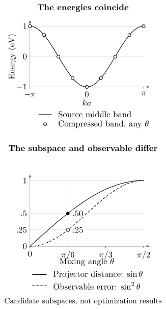
The energy curves agree for every candidate, while the projector distance and observable error grow as $\sin\theta$ and $\sin^2\theta$. At $\theta=\pi/6$, they are $0.5$ and $0.25$. These are deliberately chosen subspaces, not outputs of a localization algorithm.

The example isolates a limitation of energy-only comparisons. It does not claim that these candidates are equivalent minima of a spread functional.

Finite Fourier transforms and hopping range

On a uniform mesh of $N_k$ momenta, the chosen frame defines

$$|w_{n\mathbf R}\rangle =\frac1{\sqrt{N_k}}\sum_{\mathbf k} e^{-i\mathbf k\cdot\mathbf R}|\Phi_{n\mathbf k}\rangle.$$

This finite transform changes basis within the discrete retained space. Its continuum interpretation and localization conditions are explained in Wannier functions. In a source eigenbasis with energy matrix $\varepsilon(\mathbf k)$, compute

$$H^W(\mathbf k)=Q_{\mathbf k}^{\dagger} \varepsilon(\mathbf k)Q_{\mathbf k},$$ $$\widetilde H(\mathbf R)=\frac1{N_k}\sum_{\mathbf k} e^{-i\mathbf k\cdot\mathbf R}H^W(\mathbf k).$$

The raw coefficients repeat on the Born–von Karman superlattice for an unshifted mesh. A shift $\mathbf k_0$ introduces a phase for every superlattice vector $\mathbf T$:

$$\widetilde H(\mathbf R+\mathbf T) =e^{-i\mathbf k_0\cdot\mathbf T}\widetilde H(\mathbf R).$$

Consequently, these repeated coefficients are not an infinite decaying hopping series. Select a finite set of real-space representatives $\mathcal L$. Equivalent representatives on a boundary may share a weight; orbital centers can also affect which separation is shortest. The Wannier90 interpolation notes explain this distinction. Preserve the shift phases and absorb all weights and representative mappings into final matrices $H(\mathbf R)$. Check the file conventions before applying a weight: applying it twice changes the Hamiltonian.

For retained representatives $\mathcal S\subseteq\mathcal L$, reconstruct

$$H_{\mathcal S}(\mathbf k') =\sum_{\mathbf R\in\mathcal S} e^{i\mathbf k'\cdot\mathbf R}H(\mathbf R).$$

The full finite set must reproduce the construction samples. Keep Hermitian partners together, with $H(-\mathbf R)=H(\mathbf R)^{\dagger}$. Off-mesh accuracy still requires testing: many continuous functions share the same finite samples. Exercise 8 gives an explicit aliasing example.

Dropping terms from this finite interpolation produces the bound

$$\begin{aligned} B_H&=\sum_{\mathbf R\in\mathcal L\setminus\mathcal S} \|H(\mathbf R)\|_2,\\ \|H_{\mathcal L}(\mathbf k)-H_{\mathcal S}(\mathbf k)\|_2 &\le B_H. \end{aligned}$$

The triangle inequality proves it because each Fourier phase has unit modulus. For Hermitian reconstructions, corresponding ordered eigenvalues differ by at most $B_H$. This bounds the deliberate truncation of the represented interpolation, not its sampling error, subspace error, or underlying electronic approximation. Even $B_H=0$ says nothing about unsampled Fourier components. Refine both the construction mesh and hopping range when testing a compact tight-binding model.

Operators and velocities in a moving basis

For a translation-invariant one-body operator with source matrix $O^{\rm src}(\mathbf k)$, project consistently:

$$O^W(\mathbf k)=Q_{\mathbf k}^{\dagger} O^{\rm src}(\mathbf k)Q_{\mathbf k}.$$

Fourier transform it using the Hamiltonian convention. Position, dipole, current, and interaction calculations may require derivative, nonlocal, augmentation, or multi-momentum terms. They are not determined by the interpolated energies alone.

Velocity illustrates the issue. When the physical Bloch Hamiltonian $\widehat H_{\mathbf k}$ is differentiated in a fixed physical representation, the source matrix is

$$v^{\rm src}_\alpha =\frac1\hbar\Psi^{\dagger} (\partial_{k_\alpha}\widehat H_{\mathbf k})\Psi.$$

It is not generally the derivative of the diagonal eigenvalue matrix: the eigenvectors also vary with momentum. Project this physical matrix to obtain $v^P_\alpha=Q^{\dagger}v^{\rm src}_\alpha Q$. For an invariant selected subspace, define the frame connection $\mathcal A_\alpha=i\Phi^{\dagger}\partial_{k_\alpha}\Phi$. Then

$$\hbar v^P_\alpha =\partial_{k_\alpha}H^W -i[\mathcal A_\alpha,H^W].$$

The commutator accounts for the moving basis. In an energy eigenbasis it does not change the diagonal group velocities, but it can change interband matrix elements. Wang et al. (2006) demonstrate the importance of geometric and interband information in Wannier interpolation of Hall response.

A generic disentangled subspace need not be invariant. Hamiltonian action into the discarded space then adds terms to the displayed identity. Project and test the full source velocity instead of inferring it from $H^W$ and its internal connection alone. Nonlocal and augmentation contributions must be included in the source operator when applicable.

Comparing energies, subspaces, and observables

Evaluate source quantities at additional momenta across the full zone. Check that the test points are distinct from the construction points modulo reciprocal vectors: a shifted grid can still share points with the original. Refine locally around small gaps, avoided crossings, and Fermi pockets. A conventional path can miss the largest error.

Compare eigenvalue sets near degeneracies, where band labels can swap. Report maximum and weighted root-mean-square energy errors over the energy range of interest. The maximum reveals localized failures that an average can hide. Also check orthonormality, Hermiticity, frozen containment, and the chosen symmetries before interpreting a successful energy comparison.

For two orthonormal frames of the same rank, let the singular values of $\Phi_a^{\dagger}\Phi_b$ be $\cos\theta_j$. The angles measure the difference between their subspaces:

$$\begin{aligned} d_P&=\|P_a-P_b\|_2,\\ &=\sin\theta_{\max}. \end{aligned}$$

Internal basis rotations leave these angles unchanged. Unequal-rank orthogonal projectors have distance 1, so comparisons after increasing rank need a different question, such as containment of the smaller space. The overlap must use physical frames even when the two source windows contain different numbers of states.

Operator matrices require a basis alignment before subtraction. When the overlap is nonsingular, use its unitary polar factor

$$R_{ab}=\operatorname{polar}(\Phi_a^{\dagger}\Phi_b),$$

and compare $O_a$ with $R_{ab}O_bR_{ab}^{\dagger}$. This removes a basis rotation; it cannot remove a change of subspace. If an overlap singular value is too small for a stable correspondence, report the subspace mismatch rather than forcing an operator comparison.

For normalized test-point weights $\sum_{\mathbf k}w_{\mathbf k}=1$, define the absolute RMS difference and reference scale separately:

$$D_O^2=\sum_{\mathbf k}w_{\mathbf k} \|O_a-R_{ab}O_bR_{ab}^{\dagger}\|_F^2,$$ $$A_O^2=\sum_{\mathbf k}w_{\mathbf k}\|O_a\|_F^2.$$

The Frobenius norm sums squared matrix elements. A dimensionless comparison can use $D_O/\max(A_O,\sqrt J\,O_{\rm floor})$, with a physically chosen floor and the absolute difference reported too. This avoids meaningless pointwise percentages at zeros. For a vector operator, sum over components in both squared norms and use $\sqrt{J N_c}\,O_{\rm floor}$ for $N_c$ components.

Finally vary mesh, hopping range, starts, and plausible windows or trials separately. A stable optimization at fixed projector does not establish that another sensible subspace gives the same observables. Conversely, agreement among these numerical checks does not correct missing physics in the source Hamiltonian. In particular, a precise Kohn–Sham representation does not automatically give quasiparticle energies or the screened interactions needed for Hubbard physics in materials.

Exercises

Exercise 1: Classify the operations

Distinguish exact basis changes, subspace choices, numerical approximations, and physical reductions for: a $U(J)$ rotation; a complete finite Bloch–Wannier transform; selecting an isolated band family; entangled subspace selection; finite momentum sampling; hopping truncation; and projecting a Coulomb interaction.

Solution

A $U(J)$ rotation and the complete finite transform are exact basis changes inside the selected discrete space. An isolated family defines an exact spectral projector, but discarding its complement is a physical reduction whose usefulness depends on the observable and energy scale. Entangled selection changes the retained subspace.

Finite sampling approximates a continuous momentum problem; truncation approximates its finite interpolation. Computing the matrix $POP$ of a specified operator is exact for a given projector. Replacing full many-body dynamics by a projected Hamiltonian is generally an additional approximation. Eliminating complementary states can generate new interactions and energy dependence. Keeping all bare projected Coulomb matrix elements does not automatically include those effects.

Exercise 2: Test a normalized trial projection

Two orthonormal physical trials, projected into a three-state outer space, give

$$A=\begin{pmatrix}1&0\\0&0.20\\0&0\end{pmatrix}.$$

Compute its singular values, $\mathcal G=A^{\dagger}A$, $\kappa_2(\mathcal G)$, and $V^{(0)}$. If a chosen numerical requirement is $\sigma_{\min}\ge0.10$, what does a refined-mesh value $0.04$ establish?

Solution

The singular values are 1 and $0.20$. Therefore

$$\mathcal G=\begin{pmatrix}1&0\\0&0.04\end{pmatrix}, \qquad \kappa_2(\mathcal G)=25.$$

Both values are nonzero, and

$$V^{(0)}=\begin{pmatrix}1&0\\0&1\\0&0\end{pmatrix}.$$

The value $0.04$ fails the stated requirement but remains nonzero: it does not prove rank loss. Normalization amplifies absolute perturbations in a projected direction whose norm is small. Assess that sensitivity relative to the actual numerical errors, and reconsider the trials or available source space if necessary. Arbitrarily rescaling a trial could change the unnormalized singular value without improving its physical overlap; that is why the normalization in the question matters.

Exercise 3: Repair impossible windows

A calculation requests $J=6$. At one momentum the outer window contains five states; at another the frozen window contains seven. Explain the failures and possible repairs. Does a failed containment residual always prove this same kind of infeasibility?

Solution

Five states cannot span six independent retained directions. Widen the outer window or compute more source bands. Seven independent frozen states cannot fit inside rank six. Narrow the frozen window or increase the rank, recognizing that the latter changes the reduced model.

Containment is a separate test of the computed subspace. For example, with two available states and $J=N_{\rm fr}=1$, freezing $e_1$ is feasible. The incorrect candidate $V=e_2$ has containment residual 1, whereas $V=e_1$ has residual 0. Thus failed containment can reflect a bad result rather than an impossible count.

Exercise 4: Reconstruct and truncate a Hamiltonian

On the dimensionless mesh $k=0,\pi/2,\pi,3\pi/2$, a scalar Hamiltonian has values $2,0,-2,0\,\mathrm{eV}$. Use

$$\widetilde H(R)=\frac14\sum_k e^{-ikR}H^W(k).$$

Choose the symmetric lift $R=0,\pm1,\pm2$, dividing the self-inverse boundary class equally between $\pm2$. Find the coefficients. What goes wrong if only $R=0,1$ are retained?

Solution

The raw boundary coefficient vanishes, so the final nonzero values are

$$\begin{aligned} H(1)&=H(-1)=1\,\mathrm{eV},\\ H(0)&=H(\pm2)=0. \end{aligned}$$

They reconstruct $2\cos k\,\mathrm{eV}$ and satisfy Hermitian pairing. Discarding $R=-1$ alone gives $e^{ik}\,\mathrm{eV}$, generally complex. The omitted-term norm is $B_H=1\,\mathrm{eV}$, but the truncated scalar function is no longer a Hermitian Hamiltonian. Retain both members of each pair. Keeping $R=\pm1$ leaves zero tail within this finite model.

Exercise 5: Test the full zone

Three construction meshes give maximum path errors $0.6,0.4,0.3\,\mathrm{meV}$. Distinct full-zone test points instead give maximum errors $12.0,5.2,2.4\,\mathrm{meV}$ and RMS errors $3.8,1.4,0.7\,\mathrm{meV}$. Which meets a maximum-error target of $2\,\mathrm{meV}$? What should be refined?

Solution

None meets the target. The decreasing RMS error shows improvement, but the finest full-zone maximum still exceeds $2\,\mathrm{meV}$. Inspect the momenta with the largest errors, including nearby gaps and orbital character. Refine the construction mesh and the test sampling in those regions while keeping the physical source Hamiltonian fixed. A small path error cannot substitute for the failed full-zone comparison.

Exercise 6: Include the velocity connection

At one momentum in an invariant two-band subspace, let

$$H^W=\begin{pmatrix}0&0\\0&1\end{pmatrix}\mathrm{eV},$$ $$\partial_kH^W=\begin{pmatrix}2&0.3\\0.3&-1\end{pmatrix} \text{eV Å},$$ $$\mathcal A=\begin{pmatrix}0&0.2i\\-0.2i&0\end{pmatrix}\text{Å}.$$

Find $\hbar v=\partial_kH^W-i[\mathcal A,H^W]$. Which entries are group velocities, and what assumption prevents direct application to an arbitrary disentangled subspace?

Solution

The connection contribution is

$$-i[\mathcal A,H^W] =\begin{pmatrix}0&0.2\\0.2&0\end{pmatrix}\text{eV Å},$$

so

$$\hbar v=\begin{pmatrix}2&0.5\\0.5&-1\end{pmatrix}\text{eV Å}.$$

At this momentum $H^W$ is diagonal, so the diagonal entries divided by $\hbar$ are group velocities. The off-diagonal entry is an interband matrix element. Differentiating only eigenvalues would miss it. The identity assumes an invariant subspace. A generic disentangled projector permits Hamiltonian action into discarded states, so the full source velocity must be projected instead.

Exercise 7: Compare projectors

Two equal-rank orthonormal frames at the same momentum have overlap singular values $0.999$, $0.980$, and $0.700$. Find their projector distance. Can an internal unitary rotation reduce it below $0.05$?

Solution

The smallest singular value gives the largest principal angle:

$$d_P=\sqrt{1-0.700^2}\simeq0.714.$$

Internal rotations preserve the two projectors and all their principal angles, so they cannot reduce this difference. Even identical energy curves would not establish that the subspaces describe the same states. The windows or trials must be reconsidered if this mismatch matters for the intended observable.

Exercise 8: Find an invisible Fourier component

A scalar source band is

$$E(k)=2\cos k+0.4\cos5k\quad\mathrm{eV}.$$

Sample $k=0,\pi/2,\pi,3\pi/2$ and fit the symmetric four-point interpolation. Show that it gives $E_4(k)=2.4\cos k\,\mathrm{eV}$. Compare the two at $k=\pi/4$. Does retaining every fitted coefficient bound the remaining sampling error by zero?

Solution

On these four samples, $5k=k+2\pi j$, so $\cos5k=\cos k$. The fifth harmonic is indistinguishable from the first. The fitted coefficients are $H(\pm1)=1.2\,\mathrm{eV}$, with the other independent coefficients zero. At the new momentum,

$$\begin{aligned} E(\pi/4)&=0.8\sqrt2\,\mathrm{eV},\\ E_4(\pi/4)&=1.2\sqrt2\,\mathrm{eV}. \end{aligned}$$

Their difference is $0.4\sqrt2\,\mathrm{eV}\simeq0.566\,\mathrm{eV}$. Keeping every fitted term gives $B_H=0$ because nothing in that finite interpolation was discarded. It does not bound the aliasing error between the interpolation and the source band. Additional source samples are needed to distinguish the two functions.

References

• N. Marzari and D. Vanderbilt, “Maximally Localized Generalized Wannier Functions for Composite Energy Bands,” Physical Review B 56, 12847–12865 (1997), doi:10.1103/PhysRevB.56.12847.
• N. Marzari, A. A. Mostofi, J. R. Yates, I. Souza, and D. Vanderbilt, “Maximally Localized Wannier Functions: Theory and Applications,” Reviews of Modern Physics 84, 1419–1475 (2012), doi:10.1103/RevModPhys.84.1419.
• R. Sakuma, “Symmetry-Adapted Wannier Functions in the Maximal Localization Procedure,” Physical Review B 87, 235109 (2013), doi:10.1103/PhysRevB.87.235109.
• I. Souza, N. Marzari, and D. Vanderbilt, “Maximally Localized Wannier Functions for Entangled Energy Bands,” Physical Review B 65, 035109 (2001), doi:10.1103/PhysRevB.65.035109.
• X. Wang, J. R. Yates, I. Souza, and D. Vanderbilt, “Ab Initio Calculation of the Anomalous Hall Conductivity by Wannier Interpolation,” Physical Review B 74, 195118 (2006), doi:10.1103/PhysRevB.74.195118; erratum, Physical Review B 76, 169902 (2007), doi:10.1103/PhysRevB.76.169902.
• Wannier90 developers, “Files,” “Parameters,” and “Some Notes on the Interpolation,” Wannier90 User Guide, accessed 15 October 2026: file formats, frozen windows, finite-mesh interpolation.