DMFT for Quantum Materials

Dynamical mean-field theory, or DMFT, approximates an interacting lattice through a quantum impurity whose environment is determined self-consistently. Electrons can leave a chosen site, propagate through the surrounding solid and return. The impurity bath represents that environment, while a frequency-dependent local self-energy describes interaction effects. Self-consistency requires the impurity and the lattice to have the same local Green function.

For quantum materials, applying this idea also requires choosing correlated orbitals, screened interactions and their relation to an electronic-structure calculation. This page develops the iteration, an exact test case, and the checks needed to interpret a computed occupancy, spectrum or low-energy renormalization. Numerical convergence, accuracy of the local approximation and identification of a material phase are separate questions.

Required background. Hubbard physics in materials explains active orbitals, filling and interactions. Anderson impurity physics introduces an interacting site coupled to a noninteracting bath.

Helpful background. Thermal Green functions develops imaginary-time conventions and spectral representations.

A local self-energy can still describe dynamical correlations

In a site-local orbital basis, single-site DMFT assumes

$$\Sigma_{ia,jb}(z)=\delta_{ij}\Sigma^{(i)}_{ab}(z).$$

Here $i,j$ label sites and $a,b$ label spin and orbital modes on a site. The local matrix can have off-diagonal orbital or spin entries, and inequivalent sites can have different matrices. Single-site locality excludes intersite self-energy blocks; allowing them requires a cluster or another nonlocal approximation.

The frequency dependence is essential. A static mean field shifts levels but cannot generally describe the redistribution between coherent low-energy states and incoherent satellites. An impurity solver retains local interaction dynamics while the bath supplies electron exchange with the surrounding lattice. The approximation lies in the spatial structure of the self-energy, even when the impurity is solved very accurately.

For local-interaction lattice models with appropriately scaled hopping, the mapping becomes exact in the infinite-dimensional or infinite-coordination limit. This development began with Metzner and Vollhardt (1989) and the self-consistent impurity construction of Georges and Kotliar (1992). In a finite-dimensional material, neglected spatial correlations remain a physical approximation. Long-range interactions require additional treatment; increasing the coordination does not automatically justify discarding them.

From the lattice Green function to the next impurity bath

Use $\hbar=1$, $\beta=(k_BT)^{-1}$ and complex energy $z$. Fermionic Matsubara points are $z=i\varepsilon_n$, where

$$\varepsilon_n=(2n+1)\pi/\beta.$$

Thus $\varepsilon_n$ has energy units, and $G(z)$ has inverse-energy units. Our convention is

$$G_{ab}(\tau)=-\langle T_\tau c_a(\tau)c_b^\dagger(0)\rangle,$$

with Fourier kernel $e^{i\varepsilon_n\tau}$ on $0\leq\tau\leq\beta$.

First consider an orthonormal source Bloch basis with Hamiltonian $H^B_{\mathbf k}$. A rectangular matrix $P_{\mathbf k}$ maps source coefficients to orthonormal correlated modes, with

$$P_{\mathbf k}P_{\mathbf k}^\dagger=I.$$

For clarity, the formulas below show one correlated site per cell. With several sites, embed the separate local self-energy blocks and extract each site’s local Green function for its impurity.

In DFT+DMFT, let $V_{\rm DC}$ be the static Hermitian double-counting correction. Define

$$\begin{aligned} \Sigma_{\rm eff}(z)&=\Sigma_{\rm imp}(z)-V_{\rm DC},\\ \Lambda_{\mathbf k}(z)&=P_{\mathbf k}^\dagger \Sigma_{\rm eff}(z)P_{\mathbf k}. \end{aligned}$$

For a standalone Hubbard model without a DFT overlap correction, take $V_{\rm DC}=0$. Given a current impurity self-energy, compute

$$G^B_{\mathbf k}(z)= \left[(z+\mu)I-H^B_{\mathbf k}-\Lambda_{\mathbf k}(z)\right]^{-1},$$

and then

$$G_{\rm loc}(z)=\sum_{\mathbf k}w_{\mathbf k} P_{\mathbf k}G^B_{\mathbf k}(z)P_{\mathbf k}^\dagger,$$

where $\sum_{\mathbf k}w_{\mathbf k}=1$. The next Weiss Green function is

$$\mathcal G_{0,\rm next}^{-1}(z) =G_{\rm loc}^{-1}(z)+\Sigma_{\rm imp}(z).$$

This is the step that closes the loop. By contrast, $G_{\rm imp}^{-1}+\Sigma_{\rm imp}$ reconstructs the bath of the impurity just solved. Substituting it for $G_{\rm loc}^{-1}+\Sigma_{\rm imp}$ would simply return that old bath. Equality of the two is a result of convergence, not an identity during iteration.

The TRIQS DFTTools algorithm describes the same projection, embedding and bath update in a material calculation.

The three Green functions have different jobs. The Weiss function describes a noninteracting impurity in its bath. The impurity Green function includes the local interaction solved in that environment. The local lattice Green function averages propagation through the lattice after inserting the current self-energy. Their disagreement tells us how the environment should change. None of these is generally the Green function of an isolated atom.

For a local one-body matrix $E_{\rm imp}$, define the next hybridization by

$$\Delta_{\rm next}(z) =(z+\mu)I-E_{\rm imp}-\mathcal G_{0,\rm next}^{-1}(z).$$

Solve the impurity with this bath and the local interaction, obtain a new $G_{\rm imp}$ and $\Sigma_{\rm imp}$, and repeat. Mixing successive baths or self-energies can stabilize the iteration; the mixed object must retain the required symmetries and causal structure. At a fixed point, $G_{\rm imp}=G_{\rm loc}$ in the same basis.

A small change between successive mixed inputs is not sufficient for convergence. Very strong damping can make that change small even when the input is far from the unmixed update. Check the self-consistency residual itself. When the solver is stochastic, reducing the mixing parameter can smooth the visible trajectory without improving the underlying statistical precision.

An exact semicircular example selects the physical solution

A useful first test is a homogeneous single-band model with semicircular noninteracting density of states and half-bandwidth $D=2t_*$. For this scalar problem the bath relation is

$$\Delta(z)=t_*^2G(z).$$

It follows from the semicircular Hilbert transform and describes the usual infinite-coordination Bethe benchmark; see Georges et al. (1996). It is not the self-consistency formula for an arbitrary material Hamiltonian. For example, in a bipartite ordered Bethe solution, the bath on one sublattice depends on the Green function of the other.

Set $U=\mu=E_{\rm imp}=0$. Dyson’s equation becomes

$$G(z)=\frac1{z-t_*^2G(z)},$$

so

$$t_*^2G(z)^2-zG(z)+1=0.$$

There are two algebraic roots. Define $R(z)=\sqrt{z-2t_*}\sqrt{z+2t_*}$ in the upper half-plane using the principal square root of each factor. The physical root is

$$G_{\rm phys}(z)=\frac{2}{z+R(z)}.$$

This expression avoids subtracting nearly equal large numbers. It equals $(z-R)/(2t_*^2)$ and has $G(z)\sim1/z$. The other root, $(z+R)/(2t_*^2)$, grows like $z/t_*^2$ and has the wrong imaginary sign. Both satisfy the quadratic equation exactly. A vanishing equation residual therefore does not alone select a physical Green function.

The large-energy coefficient comes from the fermionic anticommutator: one canonical mode carries unit total spectral weight. The imaginary sign comes from a positive spectral density divided by an energy argument in the upper half-plane. These are independent physical requirements that can reject an apparently converged answer before examining any detailed spectral feature.

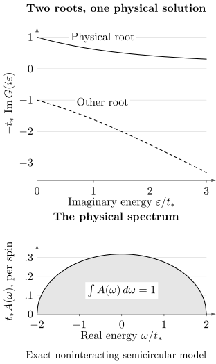
Top: on $z=i\varepsilon$ with $\varepsilon>0$, the physical root has $-\operatorname{Im}G>0$ and the correct high-energy decay. The other root also solves the quadratic equation but is unphysical. Bottom: the physical root gives a positive semicircular spectral density, normalized to one per spin. This is an exact noninteracting spectrum, not a numerical continuation or an interacting Mott spectrum.

The spectrum is

$$A(\omega)=\frac{\sqrt{4t_*^2-\omega^2}}{2\pi t_*^2} \quad (|\omega|\leq2t_*),$$

and zero outside. Here $\omega$ is real energy. Direct integration gives $\int A\,d\omega=1$, first moment zero and second moment $t_*^2$. The same normalization is used by the TRIQS semicircular Green-function implementation. These checks connect self-consistency, causality and spectral weight in a calculation whose answer is known before any many-body solver is introduced.

Correlated orbitals determine what is treated locally

A material calculation starts with a specified structure, one-body Hamiltonian, spin convention, electron count and correlated orbital frame. The orbitals should be localized enough that an onsite interaction and self-energy are meaningful approximations. The energy window, local axes and excluded bands affect this choice. Wannierization workflows explains how to construct and test the subspace and its basis.

Raw overlaps need not have orthonormal rows. With full row rank, one possible canonical analysis map is

$$\widetilde P=(PP^\dagger)^{-1/2}P.$$

Without this normalization, $PG^BP^\dagger$ has leading moment $PP^\dagger/z$, rather than $I/z$. In a nonorthogonal source, overlap matrices and dual vectors must also be included. Converting consistently to orthonormal source and local frames makes the equations above applicable; inserting an overlap matrix into only one formula does not.

Subspace agreement is necessary but not sufficient to compare local approximations. For equal ranks in a common source space, $\Pi=P^\dagger P$ gives the distance $\|\Pi_A-\Pi_B\|_2$. Yet $P'(\mathbf k)=U(\mathbf k)P(\mathbf k)$ leaves this projector unchanged. A momentum-dependent rotation can mix orbitals in different real-space cells, making an onsite self-energy or interaction nonlocal in the new frame.

A site-local, momentum-independent rotation preserves the same approximation when the interaction tensor, levels, double counting and observables are all transformed. Truncating the transformed interaction to density-density terms can break that equivalence. This distinction between a retained subspace and the local orbitals used within it is central to Lechermann et al. (2006). Even perfectly matching interpolated bands cannot settle it.

Distinguish this physical choice from merely changing coordinates in the source Bloch space. A consistent source-basis transformation changes the Hamiltonian and projectors together and leaves the represented local problem unchanged. Changing the correlated orbitals themselves can change which interaction terms or self-energy components are retained. Keeping these two operations separate makes comparisons between orbital constructions easier to interpret.

Interactions, double counting and the impurity level

The impurity interaction is an operator specified by an orbital and spin tensor. The numbers $U$ and $J$ specify it only after a parametrization has been chosen. In a rotational Kanamori parametrization, $U'=U-2J$, with spin-flip and pair-hopping terms as well as density interactions. A general crystal-field-dependent tensor need not obey that reduction. A frequency-dependent screened interaction likewise requires a solver and formulation that represent its retardation; replacing it by a static value is an additional approximation.

In DFT+DMFT, double counting adjusts interaction contributions represented both in the density-functional starting point and in the added local many-body treatment. Fully localized limit, around-mean-field and nominal prescriptions differ; a result must specify which is used. Functional-specific overlap constructions also exist, including Haule (2015). Their validity and meaning depend on the density functional, local interaction and definition of the correlated modes used in that formulation.

Our subtraction sign fixes the local level. Define

$$h_{\rm loc}=\sum_{\mathbf k}w_{\mathbf k} P_{\mathbf k}H^B_{\mathbf k}P_{\mathbf k}^\dagger.$$

For a bath with $\Delta(z)\to0$ at large $|z|$, consistency requires

$$E_{\rm imp}=h_{\rm loc}-V_{\rm DC}.$$

To see why, expand $\Sigma_{\rm imp}(z)=\Sigma_\infty+O(1/z)$. The local Green function has

$$\begin{aligned} G_{\rm loc}(z)&=I/z+M_1/z^2+\cdots,\\ M_1&=h_{\rm loc}+\Sigma_\infty-V_{\rm DC}-\mu I. \end{aligned}$$

Adding $\Sigma_{\rm imp}$ to its inverse cancels $\Sigma_\infty$. Choosing the stated $E_{\rm imp}$ then leaves a decaying hybridization. Any other choice introduces a constant that must be absorbed into the local level explicitly. Subtracting double counting again in the impurity Dyson update would count the shift twice.

Total cell filling, correlated occupancy and individual orbital occupations are different quantities. At fixed total filling, adjust $\mu$ while updating the lattice. Include contributions from any filled or empty bands treated outside the explicit source window consistently. At fixed $\mu$, changing a level shift can change the thermodynamic state.

In an isolated model where every mode is correlated, a uniform scalar level shift can be absorbed into $\mu$ at fixed filling. A shift on d orbitals alone in a p–d model instead changes their alignment relative to ligand states, and generally changes orbital populations. Exercise 4 demonstrates this distinction in a two-level model.

Consequently, convergence at one choice of interaction or relative level shift does not estimate uncertainty in that choice. First reduce numerical errors for each specified model, then compare models at matched temperature, filling and symmetry conditions. A spread caused by changing the screened interaction should not be labeled a Monte Carlo standard error.

Solvers, charge feedback and convergence

Choose an impurity solver for the actual interaction and bath matrices. The hybridization-expansion Monte Carlo method introduced by Werner et al. (2006) samples an expansion to all orders. A general local trace implementation can treat spin-flip and pair-hopping terms, but its cost and sign problem depend strongly on orbital number and basis.

The usual efficient segment implementation uses occupation intervals for a density-density local Hamiltonian and a compatible diagonal local one-body and hybridization structure. Check the implementation’s supported matrices: density-density interactions alone do not guarantee that an ordinary diagonal-bath solver is suitable. Modified segment methods can handle off-diagonal hybridization, as in Sotnikov and Kuneš (2016). Diagonalizing a bath separately at each frequency is not generally one canonical local basis transformation.

Finite-bath exact diagonalization gives poles directly but requires bath-size convergence. Additional truncation of many-body states or thermal sums is a separate possible approximation. Numerical renormalization group is particularly effective for suitable few-channel low-energy impurity problems; a realistic multiorbital calculation can be much more costly. Perturbative solvers require their own coupling regime and convergence checks.

One-shot DFT+DMFT keeps the starting density and one-body Hamiltonian fixed while closing the impurity–lattice loop. Charge-self-consistent DFT+DMFT also reconstructs the electronic density and updates the source Hamiltonian in an outer loop. The double-counting prescription and projector construction must remain consistent through those updates; a prescribed occupancy-dependent correction may itself change. Park, Millis and Marianetti (2014) discuss charge feedback and total-energy calculations. Charge self-consistency does not eliminate uncertainty in interactions or the local approximation.

Numerically, vary the momentum integration, Matsubara cutoff, tail treatment and solver controls independently. Compute correlated occupancy from

$$n_{\rm corr}=\frac1\beta\sum_n e^{i\varepsilon_n0^+} \operatorname{Tr}G_{\rm loc}(i\varepsilon_n),$$

with the analytic high-energy contribution and contact convention included. A finite sum without the missing tail can look stable while giving the wrong charge.

One practical approach subtracts a known asymptotic function before summing numerically and adds its infinite-frequency sum back analytically. The remaining summand decays faster. Increasing the cutoff then tests the small remainder, rather than repeatedly approximating a slowly convergent leading term. The moments used in the subtraction should agree with the same equal-time occupations and interactions used by the solver.

For Monte Carlo, compare independent runs, estimate autocorrelation times, and choose blocks longer than the relevant correlations. Measurement count is not effective sample size. Mean sign, acceptance and time histories help diagnose sampling, but none replaces an uncertainty estimate. Keep covariance across frequencies and orbital components when fitting or transforming the data.

The difference $\delta=g_{\rm imp}-g_{\rm loc}$, written as real components, has covariance

$$C_\delta={}C_{\rm imp}+C_{\rm loc} -C_{\rm imp,loc}-C_{\rm imp,loc}^{\mathsf T}.$$

Shared solver samples make the cross terms important. Require both small residuals in physically meaningful units and sufficiently precise estimates. Compatibility with zero through very large error bars is weak information. Checking many frequencies at a pointwise two-standard-error level is not a simultaneous test. Use a calibrated joint test or simultaneous intervals, and confirm the final solution with independent sampling or a suitable sequential procedure. A pseudoinverse covariance must not silently discard an unconverged direction.

Physical checks and limits of interpretation

For $X=G,\Delta,\Sigma$, define the Hermitian imaginary part by

$$\operatorname{Im}_{\rm H}X=(X-X^\dagger)/(2i).$$

Causality requires $-\operatorname{Im}_{\rm H}X\succeq0$ at positive Matsubara energy and for retarded boundary values. Check eigenvalues with numerical uncertainty in mind. Positive diagonal entries alone do not establish a positive semidefinite matrix.

For orthonormal correlated modes,

$$\begin{aligned} A(\omega)&=-\pi^{-1}\operatorname{Im}_{\rm H}G^R(\omega),\\ \int d\omega\,\operatorname{Tr}A(\omega)&=N_{\rm corr}. \end{aligned}$$

Check high-frequency moments, noninteracting and atomic limits, conserved filling and symmetry. Different initial self-energies can converge to distinct solutions. Compare the appropriate free energies at fixed particle number or grand potentials at fixed chemical potential before selecting a thermodynamic phase; hysteresis alone does not locate its transition.

These limits test different parts of a calculation. Switching off the interaction tests the lattice integration and bath construction. Switching off hopping tests the local levels, interaction tensor and impurity thermal weights. Neither limit alone tests the full interacting lattice calculation, but failure in either one identifies a problem that tighter iteration tolerances cannot repair.

On a differentiable Fermi-liquid branch one may define

$$Z=\left[I-\partial_\omega \operatorname{Re}_{\rm H}\Sigma^R(0)\right]^{-1}.$$

A fit to the first few finite-temperature Matsubara points is a conditional estimate of this low-energy behavior. Orbital diagonal entries depend on basis and are not automatically band residues or effective-mass ratios. Vary temperature and fit range before interpreting a small fitted slope as asymptotic physics.

Analytic continuation is needed only for quantities requiring real energy. Retain the imaginary-axis data, covariance and moments; calibrate recoverable features using synthetic data with comparable noise; and back-transform candidate spectra. Vary priors, support and regularization. Agreement between methods is useful, but shared assumptions can hide the same ambiguity. Analytic continuation develops these issues; exercise 6 gives an exact example of tiny low-energy weight that can fall below finite precision.

A good back-transform means that a candidate spectrum reproduces the supplied data within uncertainty. It does not mean that no other spectrum can do so. Feature stability is therefore a separate question: vary admissible alternatives and ask whether the particular peak, edge or integrated weight survives, rather than judging only how smooth or visually plausible one reconstruction looks.

A local spectral gap is not automatically an optical, mobility or transport gap. Intrinsic spectral functions also differ from measured photoemission intensity, which includes occupation, matrix elements and instrumental effects; see angle-resolved photoemission spectroscopy.

Finally, test important locality assumptions with aligned cluster or other nonlocal calculations when available. Momentum dependence of a spectrum alone does not establish nonlocal self-energy: the band Hamiltonian already disperses. A ratio of nonlocal to onsite self-energy norms also depends on normalization and the treatment of static parts. Compare its effect on the requested observable, keeping shared uncertainties, rather than treating every resolved nonlocal component as proof of a different phase.

Exercises

1. Select the physical quadratic root

For the noninteracting semicircular model, evaluate both roots at $z=it_*$. Which conditions select the physical one, although both have zero equation residual?

Solution

At this point $R=i\sqrt5\,t_*$, so

$$\begin{aligned} G_{\rm phys}(it_*)&=-\frac{i(\sqrt5-1)}{2t_*},\\ G_{\rm other}(it_*)&=\frac{i(\sqrt5+1)}{2t_*}. \end{aligned}$$

Their dimensionless $-t_*\operatorname{Im}G$ values are $0.618$ and $-1.618$. Only the first is causal. At high energy it approaches $1/z$, while the other grows like $z/t_*^2$. Normalization and analyticity therefore reject the second root independently of its algebraic residual.

2. Match the impurity level and high-frequency tail

Take one correlated orbital with $h_{\rm loc}=-0.50\,\mathrm{eV}$, $V_{\rm DC}=0.20\,\mathrm{eV}$, $U=2.0\,\mathrm{eV}$, $\mu=0$ and opposite-spin occupation $0.40$. Find $E_{\rm imp}$, $\Sigma_\infty$, $\Sigma_1$ and $M_1$, using the single-orbital static-interaction moment identities.

Solution

The impurity level is $-0.70\,\mathrm{eV}$. For this Hubbard interaction,

$$\begin{aligned} \Sigma_\infty&=U\bar n=0.80\,\mathrm{eV},\\ \Sigma_1&=U^2\bar n(1-\bar n)=0.96\,\mathrm{eV}^2. \end{aligned}$$

Thus $M_1=E_{\rm imp}+\Sigma_\infty=0.10\,\mathrm{eV}$. Adding the full impurity self-energy to $G_{\rm loc}^{-1}$ gives $\mathcal G_0^{-1}=z+0.70\,\mathrm{eV}+O(1/z)$. The chosen level makes $\Delta$ decay. Choosing $E_{\rm imp}=h_{\rm loc}$ instead would leave the constant $-0.20\,\mathrm{eV}$ in $\Delta$.

3. Check matrix causality

Consider $K=-\operatorname{Im}_{\rm H}\Sigma^R$ with

$$K=\begin{pmatrix}0.20&b\\b&0.10\end{pmatrix}\mathrm{eV},$$

where $b$ is dimensionless. Test $b=0.06$ and $b=0.16$.

Solution

The eigenvalues are

$$\lambda_\pm=\frac{0.30\pm\sqrt{0.01+4b^2}}2\,\mathrm{eV}.$$

For $b=0.06$, they are approximately $0.228$ and $0.072\,\mathrm{eV}$, both positive. For $b=0.16$, they are $0.318$ and $-0.018\,\mathrm{eV}$. The latter fails causality despite positive diagonals. If the matrix is estimated statistically, compare the negative eigenvalue with its uncertainty before diagnosing a significant violation.

4. Distinguish a relative shift from a common shift

One spinless electron occupies the lower eigenstate of

$$H(v)=\begin{pmatrix}1-v&0.5\\0.5&-1\end{pmatrix}\mathrm{eV}$$

in a d,p basis, with dimensionless $v$. Find its d occupation at $v=0,2,4$. Compare with a common energy shift of both orbitals.

Solution

Set $\delta=2-v$. The separation of the two levels is $\sqrt{\delta^2+1}\,\mathrm{eV}$, and the lower state’s d weight is

$$n_d=\frac12\left(1-\frac{\delta}{\sqrt{\delta^2+1}}\right).$$

The occupations are $0.0528$, $0.5000$ and $0.9472$. Lowering only the d level transfers orbital weight. In contrast, $H\mapsto H-cI$ and $\mu\mapsto\mu-c$ leave $(z+\mu)I-H$, eigenvectors and occupations unchanged. This is a two-level illustration of relative alignment, not a calculation of a bulk charge-transfer or Mott gap.

5. Choose a compatible solver

A finite-temperature three-orbital impurity has spin-flip and pair-hopping terms and an off-diagonal hybridization matrix. Can an ordinary density-density, diagonal-bath segment implementation solve it unchanged? What do general-trace CT-HYB and finite-bath diagonalization require?

Solution

No. Both the local interaction and bath structure exceed the stated implementation’s assumptions. A density-density truncation changes the interaction and still does not fix unsupported off-diagonal hybridization. Modified segment methods can support that bath structure, but this does not make the omitted spin-flip and pair-hopping terms disappear.

A general local trace CT-HYB implementation must represent the full interaction and bath, with sign, autocorrelation and cost checked. Finite-bath diagonalization can represent the same local interaction but approximates the bath by finitely many levels; test bath convergence and any additional Hilbert-space or thermal truncation separately.

6. Hide a tiny amount of low-energy spectral weight

Compare the normalized spectra

$$\begin{aligned} A_g(\omega)&=\tfrac12[\delta(\omega-a)+\delta(\omega+a)],\\ A_\eta(\omega)&=(1-\eta)A_g(\omega)+\eta\delta(\omega), \end{aligned}$$

where $a>0$ and $0<\eta<1$. Derive their Green-function difference at positive Matsubara energy. What does it imply for a hard-gap claim from finite-precision data?

Solution

The spectral representation gives $G_g(z)=z/(z^2-a^2)$ and $G_\eta=(1-\eta)G_g+\eta/z$. Consequently,

$$G_\eta(i\varepsilon)-G_g(i\varepsilon) =-\frac{i\eta a^2}{\varepsilon(\varepsilon^2+a^2)}.$$

Its magnitude is at most $\eta/\varepsilon$. At $a=0.5\,\mathrm{eV}$, $\eta=10^{-4}$ and $T=290\,\mathrm K$, the maximum difference over positive Matsubara points is about $0.00124\,\mathrm{eV}^{-1}$. Yet $A_\eta$ has weight at zero energy for every positive $\eta$. Finite uncertainty can therefore hide sufficiently small weight. This limits exact hard-gap claims; it does not prevent estimating a coarse suppression of low-energy spectral weight under stated assumptions.

7. Compare two estimates with shared uncertainty

Single-site and cluster calculations give a spectral feature at $0.31$ and $0.22\,\mathrm{eV}$, with standard errors $0.08$ and $0.10\,\mathrm{eV}$. If their correlation coefficient is $0.8$, find the standard error of the difference. What if their covariance is unknown?

Solution

For difference $D$, use

$$\begin{aligned} \operatorname{Var}D &=0.08^2+0.10^2 -2(0.8)(0.08)(0.10) \\ &=0.0036\,\mathrm{eV}^2. \end{aligned}$$

The difference is $0.09\pm0.06\,\mathrm{eV}$ at the one-standard-error level. Under an additional Gaussian approximation it is only a 1.5-standard-error displacement. Assuming independence would instead give about $0.128\,\mathrm{eV}$ for the error of the difference.

With unknown covariance, neither number is justified. Estimate paired uncertainties or retain that limitation. A resolved nonlocal self-energy component would not by itself establish a resolved shift of this feature or a different phase.

8. Check Matsubara units and a bath update

At $T=290\,\mathrm K$, find $\varepsilon_0$ and $\varepsilon_3$. For $D=2t_*=2\,\mathrm{eV}$ and $G(i\varepsilon_0)=(-0.10-0.62i)\,\mathrm{eV}^{-1}$, calculate the scalar Bethe bath update and test its sign. Assume this $G$ is a trial impurity output, not necessarily a fixed point.

Solution

Using $k_B=8.617333262\times10^{-5}\,\mathrm{eV/K}$ gives

$$\varepsilon_0\simeq0.07851\,\mathrm{eV},\qquad \varepsilon_3\simeq0.54956\,\mathrm{eV}.$$

Since $t_*=1\,\mathrm{eV}$,

$$\Delta_{\rm next}(i\varepsilon_0) =(-0.10-0.62i)\,\mathrm{eV}.$$

The dimensions are energy squared times inverse energy. The positive quantity $-\operatorname{Im}\Delta=0.62\,\mathrm{eV}$ passes this scalar causal-sign check. It does not establish that the full function is causal or that the loop has converged; those require the remaining frequencies, asymptotics and impurity–lattice comparison.

References

• A. Georges and G. Kotliar, “Hubbard model in infinite dimensions,” Physical Review B 45, 6479–6483 (1992). doi:10.1103/PhysRevB.45.6479.
• A. Georges, G. Kotliar, W. Krauth, and M. J. Rozenberg, “Dynamical mean-field theory of strongly correlated fermion systems and the limit of infinite dimensions,” Reviews of Modern Physics 68, 13–125 (1996). doi:10.1103/RevModPhys.68.13.
• K. Haule, “Exact double counting in combining the dynamical mean field theory and the density functional theory,” Physical Review Letters 115, 196403 (2015). doi:10.1103/PhysRevLett.115.196403.
• F. Lechermann, A. Georges, A. Poteryaev, S. Biermann, M. Posternak, A. Yamasaki, and O. K. Andersen, “Dynamical mean-field theory using Wannier functions: A flexible route to electronic structure calculations of strongly correlated materials,” Physical Review B 74, 125120 (2006). doi:10.1103/PhysRevB.74.125120.
• W. Metzner and D. Vollhardt, “Correlated lattice fermions in $d=\infty$ dimensions,” Physical Review Letters 62, 324–327 (1989); erratum 62, 1066 (1989). doi:10.1103/PhysRevLett.62.324.
• H. Park, A. J. Millis, and C. A. Marianetti, “Computing total energies in complex materials using charge self-consistent DFT+DMFT,” Physical Review B 90, 235103 (2014). doi:10.1103/PhysRevB.90.235103.
• A. Sotnikov and J. Kuneš, “Field-induced exciton condensation in LaCoO₃,” Scientific Reports 6, 30510 (2016). doi:10.1038/srep30510.
• TRIQS contributors, “Semicircular Green’s function,” TRIQS documentation, version 4.0.2, accessed 15 October 2026. Documentation.
• TRIQS DFTTools contributors, “Introduction to DFT+DMFT,” TRIQS DFTTools documentation, accessed 15 October 2026. Documentation.
• P. Werner, A. Comanac, L. de’ Medici, M. Troyer, and A. J. Millis, “Continuous-time solver for quantum impurity models,” Physical Review Letters 97, 076405 (2006). doi:10.1103/PhysRevLett.97.076405.