

Band Structure Workflows
A band calculation connects a crystal structure to electronic energies and states throughout the Brillouin zone. The familiar plot along a few lines is one view of those results. Finding a gap, a small Fermi pocket, or a preferred magnetic state requires additional calculations. This guide develops the sequence for periodic independent-electron and Kohn–Sham models, with an exact two-band example showing why a convincing path plot can miss metallic bands.
Required background. Crystals and lattices introduces primitive cells and fractional coordinates. Band theory introduces Bloch states, band filling, and direct versus indirect gaps.
Helpful background. Computational quantum matter explains solver, basis, and model errors. The electronic-structure methods map compares the approximations used to construct an electronic Hamiltonian.
From a crystal to a self-consistent Hamiltonian
Section titled “From a crystal to a self-consistent Hamiltonian”Start by specifying the lattice vectors, atomic species and positions, electron number, and magnetic arrangement. A magnetic unit cell can be larger than the structural primitive cell. A slab also needs a vacuum thickness and an electrostatic boundary prescription; a charged periodic cell needs a stated charge-compensation model. These choices change the physical problem.
Next choose the electronic approximation: for example a semilocal exchange-correlation functional, a core/valence partition, and scalar-relativistic or spin–orbit treatment. A plane-wave cutoff controls the accuracy of the chosen basis. Raising it cannot repair an unsuitable pseudopotential or missing correlation physics. Semicore electrons may matter for bonding, magnetism, and pressure response. Martin (2020) discusses these distinctions in detail.
In a nonorthogonal basis the band problem is
The overlap matrix is positive definite after linear dependencies have been removed. It becomes the identity for an orthonormal basis. The second equation defines normalization in this representation; Euclidean normalization of the coefficient vector generally does not suffice. PAW and ultrasoft methods also require their augmentation contributions when reconstructing densities and matrix elements (Blöchl 1994; Vanderbilt 1990).
Count each electronic state once
Section titled “Count each electronic state once”Normalize integration weights by . With occupations between zero and one for physical Fermi occupations, the electron number per cell is
Use when the two identical spin states are implicit. Use when spin channels or spinor states are enumerated explicitly, or in a spinless model. Thus two completely filled spin-degenerate bands and four filled explicit spinor bands each contain four electrons per cell. Applying both conventions at once doubles the count.
Solve the self-consistency problem
Section titled “Solve the self-consistency problem”In ordinary semilocal Kohn–Sham calculations, the input charge and spin densities determine an effective Hamiltonian. Solving it and occupying its states produces new densities. Mixing and iteration seek a fixed point of this process (Kohn and Sham 1965; Kresse and Furthmüller 1996).
An illustrative charge-density residual is
where is electron number density. A spin calculation must also monitor its magnetic degrees of freedom. Small changes in total energy alone can hide an unstable moment, occupation, or small band gap. A converged fixed point is not necessarily a minimum, and several distinct fixed points can exist.
Keep the structure, pseudopotential files, input settings, code version, and convergence histories with the resulting states. These make a calculation repeatable and help explain discrepancies between two runs.
Separate integration meshes from plotting paths
Section titled “Separate integration meshes from plotting paths”Different sets of momenta answer different questions:
| Calculation | Main task | What to refine |
|---|---|---|
| Self-consistent mesh | Determine the electronic state | Density, energy, moments |
| Dense full-zone sampling | Find extrema and count states | Gap, pockets, chemical potential |
| Plotting path | Show selected dispersions | Resolution along chosen lines |
A uniform mesh approximates a Brillouin-zone integral; its weights and shift matter as well as its dimensions (Monkhorst and Pack 1976). A path connecting selected special points is useful for seeing symmetry and dispersion (Hinuma et al. 2017), but it has no volume-integration weights. Adding more points to the same path cannot find an extremum elsewhere.
For a converged semilocal calculation, evaluate a denser mesh and a display path using the same effective Hamiltonian. This is often called non-self-consistent, or NSCF, work. If finer integration reveals a significant change in the density or magnetic state, improve the self-consistent calculation too. A dense output grid cannot undo an inaccurate input state.
The required saved information depends on the method. Hybrid exchange depends on occupied orbitals, not only on the charge density; orbital-dependent functionals and calculations likewise require additional state data. Follow the method’s implementation instructions when constructing its fixed operator or band outputs. For example, the VASP hybrid-band instructions require regular-mesh orbitals and explicitly distinguish their procedure from a charge-density-only NSCF calculation.
Determine the chemical potential from a full-zone mesh at the required electron number. Its estimate can change as the integration is refined even when the Hamiltonian is fixed. A path plot should use that mesh-based reference, as explained in the VASP Fermi-energy documentation. At zero temperature in an insulator, any chemical potential inside the global gap gives the same filling; state the plotting convention used.
A path can miss an indirect band overlap
Section titled “A path can miss an indirect band overlap”For two adjacent energy-ordered bands, distinguish
from
The first compares states at the same momentum. The second permits different momenta and decides whether these band ranges overlap. Neither is automatically the fundamental interacting gap or an optical absorption threshold; see band gaps.
Consider a spinless two-orbital lattice model, with lattice spacing set to one:
Here are dimensionless and periodic modulo . The square translation lattice does not imply fourfold rotation symmetry for this Hamiltonian. Its two eigenvalues are , so the direct separation is exactly everywhere.
Now plot the chosen path , , , then back to . On the first two segments . On the diagonal, putting gives
Its largest magnitude is . The path therefore suggests a positive separation between the two band ranges:
Elsewhere in the zone, reaches . For example, the lower band has its maximum at ; the upper band has its minimum at . Both points are away from the plotted path. The actual indirect gap is : the band ranges overlap.
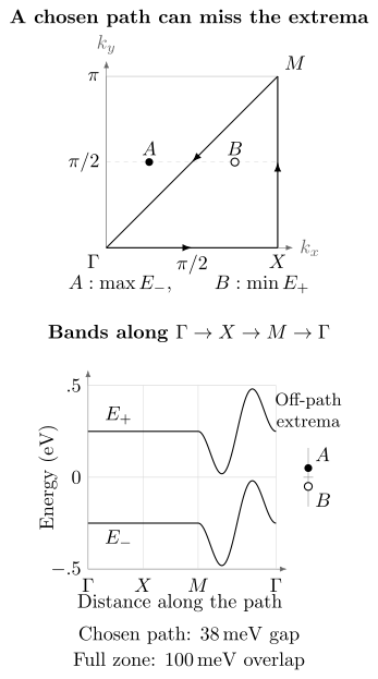
Exact results for the two-orbital model. The path shows a separation; the full zone has a overlap. The marked extrema lie in the displayed quadrant; the model is periodic over the full zone. The horizontal plot coordinate is distance along the path.
At one electron per cell, zero-temperature equilibrium fills all states below a common chemical potential. Here symmetry gives , with electron and hole pockets. Filling the entire lower band and none of the upper band would instead occupy some states above empty, lower-energy states. In a self-consistent material calculation, discovering such an overlap requires reconsidering any imposed insulating occupations and recalculating the state. The frozen-Hamiltonian overlap is a warning, not by itself a completed self-consistent semimetal calculation.
Converge the quantity you need
Section titled “Converge the quantity you need”A total energy can be stable before a small gap, a pocket volume, or a band curvature is resolved. Vary the basis cutoff, self-consistent mesh, output mesh, and solver tolerance separately, then check that tightening them together does not expose a missed dependence. For structural relaxation, also check forces and stress: a changing basis can cause Pulay errors.
There is a useful exact statement for a fixed Hamiltonian. If extrema are searched only over a set of momenta, then
Adding samples can only lower this sampled gap. Preserve previously found extrema when refining the search. Grids with different shifts or nonnested sizes can fluctuate, but a later grid does not invalidate an earlier, more restrictive bound. If the Hamiltonian changes during a new self-consistent calculation, this monotonic argument no longer applies between the runs.
For the model above, nested grids with coordinates , , give:
| Sampled indirect gap (meV) | |
|---|---|
| 6 | |
| 12 | |
| 24 | |
| 48 |
The coarsest grid misses the overlap. The 24-point grid happens to contain the exact extrema. In a general calculation, two similar successive values do not prove an error bound: search near candidate extrema and test alternative mesh shifts or adaptive refinement. Numerical stability and a rigorous bound are different conclusions.
Compare uncertainty sources separately. Mesh and basis changes measure numerical sensitivity. A new functional, valence partition, structure, or magnetic arrangement changes the model or physical input. Agreement between codes solving the same approximate equations is valuable, but does not remove their shared approximation (Lejaeghere et al. 2016).
Treat occupations and magnetism consistently
Section titled “Treat occupations and magnetism consistently”Smearing has a specific purpose
Section titled “Smearing has a specific purpose”For Fermi–Dirac occupations,
Using a numerical width smooths integration across a Fermi surface. Interpreting it as a physical temperature requires a finite-temperature model; it is not a quasiparticle lifetime or an instrumental resolution. The internal energy, the free energy minimized by the calculation, and a code’s extrapolated zero-width energy are distinct quantities. With physical Fermi–Dirac entropy expressed in units of , .
For a smooth density of states and a stable branch, an internal-energy difference can have a leading correction. This motivates testing at small widths. It does not justify that fit near every singularity, phase change, or poorly resolved pocket. Refine the momentum mesh as the width decreases.
Methfessel–Paxton and cold-smearing schemes use different occupation and entropy functions. Their occupations can be nonmonotonic, so electron counting can admit several chemical-potential roots; dos Santos and Marzari (2023) explain this problem and root-selection methods. Do not transfer a Fermi–Dirac extrapolation rule to a different scheme without checking it. Fixed integer occupations are appropriate only after the assumed insulating filling is consistent with the spectrum throughout the zone.
Compare several magnetic solutions
Section titled “Compare several magnetic solutions”Try physically motivated nonmagnetic, ferromagnetic, antiferromagnetic, and, where relevant, noncollinear initial states. Several initial moment sizes help find distinct self-consistent solutions. A small cell excludes orders that require larger periods; spin–orbit coupling can make the moment direction matter.
Compare the same composition with a stated normalization:
where each counts atoms or formula units consistently. Match the structural protocol, basis accuracy, reciprocal sampling density, and occupation/energy conventions. If comparing relaxed phases, relax each under a common protocol; if comparing spin states at fixed geometry, keep that geometry fixed.
Suppose a teaching calculation gives AFM minus FM energy differences of with PBE and with PBEsol. Here the allowances apply to the relative energies and summarize numerical sensitivity, not statistical confidence. Both signs are numerically stable, yet the two approximations favor different states. More precise diagonalization cannot resolve that model dependence. The PBE and PBEsol definitions are given by Perdew et al. (1996, 2008).
Spinful time-reversal symmetry also constrains band filling. Kramers degeneracy and, in some space groups, larger connected band groups can prohibit a symmetric band insulator at a proposed filling (Watanabe et al. 2016). A small numerical gap then calls for checking symmetry breaking, the electron count, and omitted bands. See symmetry of Bloch states.
Read more than the band energies
Section titled “Read more than the band energies”Energy ordering is appropriate when defining the gap between adjacent bands. Following an orbital character through a crossing is a different task. Near degeneracy, individual eigenvectors may rotate within a stable subspace; compare projectors or singular values of the complex overlap matrix. Squared overlap magnitudes alone lose phase information. A swap of dominant orbital character can occur at an avoided crossing as well as an exact crossing.
For an isolated differentiable band with , differentiating the generalized eigenproblem gives its group velocity:
Here is a physical wavevector component. At a degeneracy, resolve the directional derivative within the degenerate subspace. This formula for a diagonal group velocity is not a general prescription for interband optical matrix elements.
Density of states and Fermi surfaces need full-zone sampling. Orbital weights, projected densities of states, and local magnetic moments depend on the chosen projectors and spatial partition. Unfolded bands also depend on a primitive reference cell. A smooth broadened plot is not a convergence test or a many-body spectral function.
For localized interpolation, retain the states, overlap conventions, and energy range needed by Wannierization. For comparison with photoemission, use the spectral-function description and the matrix elements, surface effects, and resolution discussed in ARPES. These additional ingredients explain why a calculated band separation and a measured peak separation need not represent the same quantity.
Exercises
Section titled “Exercises”1. Count electrons with two conventions
Section titled “1. Count electrons with two conventions”An irreducible mesh has weights , , and . Two spin-degenerate bands are filled at every point. Find the electron count, then repeat for four explicitly enumerated filled spinor bands.
Solution
The weights sum to one. In the first convention ; in the second . Counting a spin degeneracy in addition to the four spinor bands would incorrectly give eight.
2. Find what the path missed
Section titled “2. Find what the path missed”For the two-orbital model, derive the diagonal-path extrema and the true indirect gap. Explain why increasing only the number of path points cannot correct the inferred sign.
Solution
Write . On the diagonal , whose stationary points have . Thus the path extrema are . The path gap is approximately , whereas the full-zone range gives . More path points converge the wrong search domain. The common chemical potential requires holes near the lower-band maximum and electrons near the upper-band minimum at one electron per cell.
3. Keep earlier extrema when refining
Section titled “3. Keep earlier extrema when refining”A fixed Hamiltonian gives sampled gaps 14, 18, and 19 meV on three nonnested meshes. What follows about the true gap? What changes if the meshes are nested? Does any of this prove that the true gap is positive?
Solution
Each sampled minimum is at least the true minimum, and each sampled maximum is at most the true maximum. Consequently each sampled gap is an upper bound, so the true gap is at most 14 meV. Searching the union can lower that bound further; it cannot raise it. A 14, 18, 19 sequence on nested meshes would contradict exact extrema sampling for the same Hamiltonian. Numerical solver errors or a changed Hamiltonian would need separate consideration.
An upper bound of 14 meV does not establish positivity: an unsampled point could still close or reverse the gap. A positive lower bound would need additional control of interpolation or variation between samples.
4. Interpret a smearing extrapolation
Section titled “4. Interpret a smearing extrapolation”Internal-energy differences at Fermi–Dirac widths 0.20, 0.10, and 0.05 eV are 8.00, 11.00, and 11.75 meV per atom. Fit a quadratic in the width and explain what the fit establishes.
Solution
With , all three points satisfy
The fitted intercept is . Exact agreement of three teaching values does not establish an asymptotic regime. Check smaller widths, denser meshes, the energy definition, and continuity of the magnetic solution before interpreting this as a reliable zero-width result.
5. Normalize a generalized eigenvector
Section titled “5. Normalize a generalized eigenvector”Solve for and . Give normalized eigenvectors.
Solution
The energies are 1 and 2 eV. Suitable coefficient vectors are and ; they satisfy . Reading the diagonal entries of as energies without including would give the wrong second energy.
6. Separate energy order from orbital character
Section titled “6. Separate energy order from orbital character”Study , where is a wavevector, has units of energy times length, and is an energy. Does a swap in the dominant orbital of the lower-energy eigenstate imply a band crossing?
Solution
The energies are , so the minimum separation is . The lower state has : its dominant orbital changes as changes sign, despite an avoided crossing. Energy order stays well defined. When , the degeneracy at requires treating the two-dimensional eigenspace there rather than assigning a unique eigenvector.
7. Test the group-velocity formula
Section titled “7. Test the group-velocity formula”For a one-dimensional nonorthogonal one-band model, take and , with . Derive the energy and velocity, retaining the overlap derivative.
Solution
The normalized coefficient has and . Direct differentiation gives
The generalized formula gives the same result because and . Omitting the overlap derivative would instead leave only one power of in the denominator. The condition on ensures a positive overlap everywhere.
References
Section titled “References”- Blöchl, P. E. “Projector Augmented-Wave Method.” Physical Review B 50, 17953–17979 (1994). doi:10.1103/PhysRevB.50.17953.
- dos Santos, F. J., and Marzari, N. “Fermi Energy Determination for Advanced Smearing Techniques.” Physical Review B 107, 195122 (2023). doi:10.1103/PhysRevB.107.195122; author manuscript.
- Hinuma, Y., Pizzi, G., Kumagai, Y., Oba, F., and Tanaka, I. “Band Structure Diagram Paths Based on Crystallography.” Computational Materials Science 128, 140–184 (2017). doi:10.1016/j.commatsci.2016.10.015.
- Kohn, W., and Sham, L. J. “Self-Consistent Equations Including Exchange and Correlation Effects.” Physical Review 140, A1133–A1138 (1965). doi:10.1103/PhysRev.140.A1133.
- Kresse, G., and Furthmüller, J. “Efficient Iterative Schemes for Ab Initio Total-Energy Calculations Using a Plane-Wave Basis Set.” Physical Review B 54, 11169–11186 (1996). doi:10.1103/PhysRevB.54.11169.
- Lejaeghere, K., et al. “Reproducibility in Density Functional Theory Calculations of Solids.” Science 351, aad3000 (2016). doi:10.1126/science.aad3000.
- Martin, R. M. Electronic Structure: Basic Theory and Practical Methods, 2nd ed. Cambridge University Press (2020). doi:10.1017/9781108555586.
- Monkhorst, H. J., and Pack, J. D. “Special Points for Brillouin-Zone Integrations.” Physical Review B 13, 5188–5192 (1976). doi:10.1103/PhysRevB.13.5188.
- Perdew, J. P., Burke, K., and Ernzerhof, M. “Generalized Gradient Approximation Made Simple.” Physical Review Letters 77, 3865–3868 (1996). doi:10.1103/PhysRevLett.77.3865.
- Perdew, J. P., et al. “Restoring the Density-Gradient Expansion for Exchange in Solids and Surfaces.” Physical Review Letters 100, 136406 (2008). doi:10.1103/PhysRevLett.100.136406.
- Vanderbilt, D. “Soft Self-Consistent Pseudopotentials in a Generalized Eigenvalue Formalism.” Physical Review B 41, 7892–7895 (1990). doi:10.1103/PhysRevB.41.7892.
- VASP developers. “Band-Structure Calculation Using Hybrid Functionals” and “EFERMI.” VASP Wiki, accessed 15 October 2026. Hybrid-band instructions; Fermi-energy instructions.
- Watanabe, H., Po, H. C., Vishwanath, A., and Zaletel, M. “Filling-Enforced Gaplessness in Band Structures of the 230 Space Groups.” Physical Review Letters 117, 096404 (2016). doi:10.1103/PhysRevLett.117.096404.