Graphene and Dirac Materials

Graphene turns a two-site crystal basis into a two-component Dirac equation. Near either of its two inequivalent band crossings, an electron’s amplitudes on the carbon sublattices behave as a pseudospin. This produces a linear dispersion, suppressed scalar backscattering and a distinctive magnetic spectrum with a zero Landau level.

The electrons remain nonrelativistic particles in a solid; the Dirac equation is a low-energy band approximation. We develop that approximation, its thermal response and its magnetic levels, then identify how masses, disorder and stacking change the predictions. Graphene Dirac Model provides a compact formula reference.

Required background. Tight-Binding Models supplies hopping matrices, Bloch’s Theorem supplies crystal momentum, Berry Phase supplies geometric phase, and Landau Levels supplies the oscillator method for magnetic quantization.

Honeycomb orbitals and the two valleys

Three in-plane bonds per carbon form the strong $\sigma$ bands. The remaining $p_z$ orbital forms the low-energy $\pi$ bands. The honeycomb network has a triangular Bravais lattice with two sites, $A$ and $B$, in each primitive cell. A spinless Bloch state therefore needs two amplitudes.

Distinguish the carbon–carbon bond length $a_0\simeq0.142\,\mathrm{nm}$ from the triangular lattice constant

$$a=\sqrt3a_0\simeq0.246\,\mathrm{nm}.$$

For nearest-neighbor hopping $t>0$, in an orbital-position Bloch convention,

$$h(\mathbf k)=-t \begin{pmatrix}0&f(\mathbf k)\\f^*(\mathbf k)&0\end{pmatrix},$$ $$f(\mathbf k)=\sum_{j=1}^3e^{i\mathbf k\cdot\boldsymbol\delta_j},$$ $$E_\pm=\pm t|f|.$$

Choose nearest-neighbor vectors

$$\boldsymbol\delta_1=a_0(0,1),$$ $$\boldsymbol\delta_{2,3}=a_0(\mp\sqrt3/2,-1/2).$$

The three phases cancel at the two inequivalent valleys

$$\mathbf K_\eta=\left(\eta\frac{4\pi}{3a},0\right), \qquad \eta=\pm1.$$

Expanding at $\mathbf k=\mathbf K_\eta+\mathbf q$ gives

$$f\simeq-\frac{3a_0}{2}(\eta q_x-iq_y),$$

and hence

$$H_\eta=\hbar v_F(\eta q_x\sigma_x+q_y\sigma_y),$$ $$v_F=\frac{3ta_0}{2\hbar}.$$

The Pauli matrices act on $(A,B)$, not real spin. The eigenvalues are $E_s=s\hbar v_Fq$, with $s=\pm1$. Real spin approximately doubles the valley multiplicity, giving $g=4$. A representative velocity is $10^6\,\mathrm{m/s}$; its value depends on hopping and renormalization, not a fundamental speed limit (Castro Neto and colleagues, 2009).

The linear expansion needs $qa_0\ll1$. Away from the valleys the full lattice dispersion matters. Time reversal exchanges the valleys; smooth disorder approximately preserves them, while atomic defects and some edges mix them. Two locally useful cones must be retained when counting states or discussing global topology.

Density, mass and thermal charge response

Measure energy from the touching and let signed density $n_s$ mean excess electrons relative to neutrality. At zero temperature,

$$|n_s|=\frac{gk_F^2}{4\pi}, \qquad |E_F|=\hbar v_Fk_F.$$

Differentiating the number of states inside the momentum disk gives the density of states per unit area

$$D(E)=\frac{g|E|}{2\pi\hbar^2v_F^2}.$$

It vanishes at the ideal touching. The cyclotron mass, obtained from the derivative of orbit area, is nevertheless meaningful away from neutrality:

$$\begin{aligned} m_c(E)&=\frac{\hbar^2}{2\pi}\left|\frac{dA_k}{dE}\right|\\ &=\frac{|E|}{v_F^2}. \end{aligned}$$

This energy-dependent orbit mass is different from a constant band-edge curvature mass; see Effective Mass. For $n_s=10^{12}\,\mathrm{cm}^{-2}$ and $v_F=10^6\,\mathrm{m/s}$, $E_F=0.117\,\mathrm{eV}$ and $m_c=0.0205m_e$.

Quantum capacitance at neutrality

The quantum capacitance per area, $c_Q=C_Q/A$, measures how charge changes with chemical potential. For the fixed noninteracting spectrum,

$$c_Q=e^2\frac{\partial n_s}{\partial\mu}$$ $$c_Q=e^2\int D(E)[-f'(E-\mu)]\,dE,$$

where $f(x)=[e^{x/(k_{\mathrm B}T)}+1]^{-1}$. The frequently used expression $c_Q=e^2D(E_F)$ is its zero-temperature limit. At finite temperature, define $x=\mu/(k_{\mathrm B}T)$ and the capacitance scale

$$c_T=\frac{ge^2k_{\mathrm B}T}{\pi\hbar^2v_F^2}.$$

Integrating the cone DOS gives

$$c_Q=c_T\ln[2\cosh(x/2)].$$

At neutrality, $c_Q(0,T)=c_T\ln2$ remains positive.

Thermally excited electrons and holes cancel in the net density at $\mu=0$, but both respond when $\mu$ changes. Temperature broadens this occupation response; it does not by itself broaden a fixed one-particle DOS (Fang and colleagues, 2007).

The measured gate capacitance also includes electrostatics; an ideal planar device has $c_{\rm gate}^{-1}=c_{\rm geom}^{-1}+c_Q^{-1}$. Traps, density puddles and interactions can require a more elaborate model. Similarly, a resistance maximum near neutrality is not a universal minimum conductivity: its height depends on contacts, geometry, disorder and temperature.

Pseudospin, backscattering and Berry phase

Write $\mathbf q=q(\cos\phi,\sin\phi)$. In the convention above, a normalized massless eigenvector is

$$|u_{s\eta}\rangle=\frac1{\sqrt2} \begin{pmatrix}1\\s\eta e^{i\eta\phi}\end{pmatrix}.$$

Its in-plane pseudospin rotates with momentum. For scalar scattering within one band and valley, write the deflection angle as $\vartheta=\phi'-\phi$. The spinor factor in the Born probability is

$$|\langle u(\phi')|u(\phi)\rangle|^2 =\frac{1+\cos\vartheta}2.$$

It vanishes at exact reversal. This suppresses one scattering process, not all resistance: other angles still relax current, and intervalley or sublattice-dependent perturbations evade the argument.

At normal incidence on a one-dimensional scalar potential, the massless continuum Hamiltonian conserves the relevant pseudospin. Its right- and left-moving states have opposite pseudospins, so reflection is forbidden even across a $p$–$n$ junction. This is the ideal Klein-transmission result (Katsnelson, Novoselov and Geim, 2006). The device must avoid intervalley mixing and mass terms. Smoothness on the lattice scale helps preserve the valley; perfect normal-incidence transmission does not additionally require slow variation on the Fermi wavelength.

For a counterclockwise loop around a valley and Berry connection $i\langle u|\nabla_{\mathbf q}u\rangle$, the massless spinor gives

$$\gamma_\eta=-\eta\pi\pmod{2\pi}.$$

The two signs represent the same phase modulo $2\pi$. A local $\pi$ phase does not make gapless graphene an insulator with a quantized bulk invariant: the touching prevents separating a globally isolated occupied band.

A mass changes more than the loop phase

A sublattice energy difference adds $\Delta\sigma_z$ and opens a gap $2|\Delta|$. The pseudospin tilts out of plane. For a circular conduction-band loop at $E>|\Delta|$,

$$\gamma_\eta(E)=-\eta\pi\left(1-\frac\Delta E\right) \pmod{2\pi}.$$

For the massless cone, the semiclassical rule may be written

$$\frac{A_k(E)\ell_B^2}{2\pi} =N+\frac12-\frac\gamma{2\pi},$$

with an integer $N$, $\ell_B=\sqrt{\hbar/(eB)}$, and positive perpendicular field magnitude $B$. The $\pi$ phase cancels the half offset modulo an integer. This is consistent with the exact zero mode derived below, although semiclassical reasoning alone is not a controlled small-index derivation.

Do not insert the massive loop phase into that unchanged formula. A massive wavepacket also has an orbital magnetic moment, which shifts its energy at the same semiclassical order. In the particle–hole-symmetric massive Dirac model, this contribution cancels the energy-dependent part of the Berry-phase offset (Fuchs and colleagues, 2010). The exact magnetic spectrum makes the cancellation testable.

Experimental fan intercepts additionally depend on level indexing, chemical-potential motion, unresolved frequencies and Zeeman splitting. An intercept alone therefore does not measure a unique Berry phase.

Landau levels and their sublattice zero modes

Take an electron of charge $-e$ with $e>0$ and first choose $B_z=B>0$. Its kinetic momentum is $\boldsymbol\pi=\mathbf p+e\mathbf A$, so $[\pi_x,\pi_y]=-ie\hbar B$. Define

$$\hat a=\frac{\ell_B(\pi_x-i\pi_y)}{\sqrt2\hbar},$$

which satisfies $[\hat a,\hat a^\dagger]=1$, and the energy scale $\epsilon_B=\sqrt2\hbar v_F/\ell_B$. Including the mass, the $\eta=+1$ valley becomes

$$H_+= \begin{pmatrix}\Delta&\epsilon_B\hat a\\ \epsilon_B\hat a^\dagger&-\Delta\end{pmatrix}.$$

For $n\ge1$, the amplitudes $A|n-1\rangle$ and $B|n\rangle$ form a closed two-state problem with off-diagonal element $\epsilon_B\sqrt n$. Its energies are

$$E_{n,\pm}=\pm\sqrt{\Delta^2+n\epsilon_B^2}.$$

There is also an unpaired state $(0,|0\rangle)^T$ with energy $-\Delta$, because $\hat a|0\rangle=0$. In the other valley the ladder operators interchange, leaving $(|0\rangle,0)^T$ at $+\Delta$. Thus

$$E_{0,\eta}=-\eta\Delta\qquad(B_z>0).$$

Reversing the field interchanges the sublattices and gives $E_{0,\eta}=-\eta\operatorname{sgn}(B_z)\Delta$. At $\Delta=0$, both zero modes remain at zero, while the other levels scale as $\pm\sqrt{nB}$ (Goerbig, 2011).

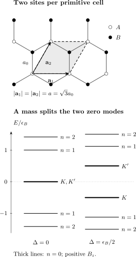
Top: the outlined primitive cell has two carbon sites after boundary sharing; $a_0$ is a bond length and $|\mathbf a_1|=|\mathbf a_2|=a=\sqrt3a_0$. Open and filled circles distinguish sublattices. Bottom: calculated levels at a fixed positive field, in units of $\epsilon_B$. A mass $\Delta=\epsilon_B/2$ shifts the zero modes to opposite energies in the two valleys. The $n\ge1$ levels remain valley-degenerate, and every level retains the passive real-spin multiplicity of the model.

For $n\ge1$, the zero-field massive orbit area is

$$A_k(E)=\frac{\pi(E^2-\Delta^2)}{\hbar^2v_F^2}.$$

Inserting the exact levels gives $A_k(E_n)\ell_B^2/(2\pi)=n$, with no energy-dependent offset. This explicit result is the useful check on the preceding Berry-phase discussion; it relies on this ideal two-band Hamiltonian.

Degeneracy and the Hall sequence

Each spin and valley supplies $eB/h$ orbital states per unit area. For unresolved massless graphene levels, the multiplicity is four. Relative to neutrality, filling the remaining half of the zero level gives $\nu=2$, and each next conduction level adds four. Holes give the opposite sequence:

$$\nu=\pm4\left(N+\frac12\right), \qquad N=0,1,2,\ldots.$$

Thus the plateau filling numbers are $\pm2,\pm6,\pm10,\ldots$; the total Hall response is an integer multiple of $e^2/h$, with sign set by the tensor convention. The sequence was observed in monolayer graphene (Zhang and colleagues, 2005). Zeeman effects, masses or interactions can resolve additional plateaus. Integer Quantum Hall Effect explains the localization and edge physics needed for finite-width plateaus; Fractional Quantum Hall Effect treats interaction-driven fractions.

Changes to the ideal material model

Added ingredient	Main change to test
Same-sublattice hopping	Electron–hole asymmetry; no necessary gap
Sublattice potential	Gap, tilted pseudospin and valley zero-mode splitting
Smooth scalar disorder	Density variations and intravalley scattering
Atomic defects or certain edges	Valley mixing
Strain or substrate alignment	Changed velocities, valley fields or superlattice potential
Electron interactions	Renormalized velocity and possible ordered states

Spectroscopy can test dispersion and gaps; capacitance probes the thermal charge response; magnetic spectroscopy tests the level ladder. Combining them helps separate a gap from density inhomogeneity or contact effects. The dimensionless Coulomb scale $e^2/(4\pi\epsilon\hbar v_F)$ depends on the dielectric environment, so a fitted velocity need not be independent of density or energy window.

Other Dirac materials need their own interpretation. A topological-insulator surface mixes spin and orbital character and is constrained by its three-dimensional bulk. Weyl and Dirac semimetals have three-dimensional nodes and different degeneracies and symmetries. The shape of a cone does not specify its components or protection.

From a monolayer to moiré bands

Twisting two graphene layers by $\theta$ gives, for equal lattice constants,

$$L_M=\frac{a}{2\sin(\theta/2)},$$ $$A_M=\frac{\sqrt3}{2}L_M^2.$$

Here $a$ is the Bravais lattice constant, not the carbon bond length. The displaced valley momenta have separation $k_\theta=2K\sin(\theta/2)$, with $K=4\pi/(3a)$. Interlayer tunneling of scale $w$ competes with $\hbar v_Fk_\theta$; their ratio controls the continuum model and can produce strongly reduced velocities and narrow bands (Bistritzer and MacDonald, 2011).

Geometry fixes the density $1/A_M$ per carrier per cell, but does not determine ordering or pairing. Moiré Superlattices develops the coupled-layer model and its limitations. The Graphene material guide compares substrate, strain and proximity modifications of the baseline derived here.

Exercises

1. Density and thermal response. For $g=4$ and $v_F=10^6\,\mathrm{m/s}$, find $k_F$ and $\lambda_F$ at $n_s=10^{12}\,\mathrm{cm}^{-2}$. What is $c_Q$ at neutrality and $300\,\mathrm K$ in the ideal cone model?

Solution

Convert $n_s$ to $10^{16}\,\mathrm m^{-2}$. Then

$$\begin{aligned} k_F&=\sqrt{\pi n_s}\\ &=1.77\times10^8\,\mathrm m^{-1}, \end{aligned}$$

and $\lambda_F=2\pi/k_F=35.4\,\mathrm{nm}$. At neutrality,

$$c_Q=\frac{4e^2k_{\mathrm B}(300\,\mathrm K)\ln2} {\pi\hbar^2v_F^2}$$

is $8.44\times10^{-3}\,\mathrm{F/m^2}$, or $0.844\,\mu\mathrm{F/cm^2}$. A zero ideal DOS at one energy does not imply a zero finite-temperature charge response.

2. Restore backscattering with a mass. For positive-energy states of the massive cone at opposite momenta, show that the scalar spinor overlap probability is $\Delta^2/E^2$.

Solution

The conduction-band pseudospin is the unit vector along $(\eta\hbar v_Fq_x,\hbar v_Fq_y,\Delta)$. Opposite momenta reverse its first two components but preserve its third. Their dot product is

$$\mathbf n_{\mathbf q}\cdot\mathbf n_{-\mathbf q} =-1+\frac{2\Delta^2}{E^2}.$$

Two spin-$1/2$ state projectors have overlap $(1+\mathbf n\cdot\mathbf n')/2$, giving $\Delta^2/E^2$. At $E=2|\Delta|$ it is $1/4$; as $\Delta\to0$ it vanishes. This is the internal-state factor, not a complete scattering rate.

3. Find both zero modes. At $B_z>0$, the second-valley matrix is

$$H_-= \begin{pmatrix}\Delta&-\epsilon_B\hat a^\dagger\\ -\epsilon_B\hat a&-\Delta\end{pmatrix}.$$

Find its zero-oscillator state and compare it with $H_+$. What does reversing the field do?

Solution

Since $\hat a|0\rangle=0$, the state $(|0\rangle,0)^T$ is an eigenstate of $H_-$ at $+\Delta$ and occupies $A$. In $H_+$, $(0,|0\rangle)^T$ has energy $-\Delta$ and occupies $B$. Reversing $B_z$ interchanges the lowering and raising roles, reversing these assignments. Setting $\Delta=0$ places both at zero energy.

4. Berry phase is not the whole orbit shift. Take $\eta=-1$, $\Delta>0$ and a conduction orbit at $E=2\Delta$. Compare the Berry-only offset with the exact massive Landau relation.

Solution

The counterclockwise phase is $\gamma=\pi/2$. Keeping only this phase would give

$$\frac12-\frac\gamma{2\pi}=\frac14.$$

But the exact levels obey

$$\begin{aligned} \frac{A_k(E_n)\ell_B^2}{2\pi} &=\frac{E_n^2-\Delta^2}{\epsilon_B^2}\\ &=n. \end{aligned}$$

The omitted orbital-moment contribution cancels the $1/4$ in this model. A measured index shift cannot generally be identified with the Berry phase alone.

5. Moiré length and density. Use $a=0.246\,\mathrm{nm}$ and $\theta=1.10^\circ$ to estimate $L_M$ and the density of four carriers per moiré cell. What error follows from substituting $a_0$ instead?

Solution

The angle is $0.01920$ radians. The geometry gives $L_M=12.8\,\mathrm{nm}$ and $A_M=142\,\mathrm{nm}^2$, hence

$$\begin{aligned} n_4&=\frac4{A_M}\\ &=2.81\times10^{12}\,\mathrm{cm}^{-2}. \end{aligned}$$

Using $a_0=a/\sqrt3$ reduces the inferred cell area by three and overestimates the filling density by three. The correct geometric density still says nothing by itself about a gap or superconductivity.

References

• R. Bistritzer and A. H. MacDonald, “Moiré Bands in Twisted Double-Layer Graphene,” Proceedings of the National Academy of Sciences 108, 12233–12237 (2011), doi:10.1073/pnas.1108174108, arXiv:1009.4203.
• A. H. Castro Neto, F. Guinea, N. M. R. Peres, K. S. Novoselov and A. K. Geim, “The Electronic Properties of Graphene,” Reviews of Modern Physics 81, 109–162 (2009), doi:10.1103/RevModPhys.81.109, arXiv:0709.1163.
• T. Fang, A. Konar, H. Xing and D. Jena, “Carrier Statistics and Quantum Capacitance of Graphene Sheets and Ribbons,” Applied Physics Letters 91, 092109 (2007), doi:10.1063/1.2776887, author-hosted paper.
• J.-N. Fuchs, F. Piéchon, M. O. Goerbig and G. Montambaux, “Topological Berry Phase and Semiclassical Quantization of Cyclotron Orbits for Two Dimensional Electrons in Coupled Band Models,” European Physical Journal B 77, 351–362 (2010), doi:10.1140/epjb/e2010-00259-2, arXiv:1006.5632.
• M. O. Goerbig, “Electronic Properties of Graphene in a Strong Magnetic Field,” Reviews of Modern Physics 83, 1193–1243 (2011), doi:10.1103/RevModPhys.83.1193, arXiv:1004.3396.
• M. I. Katsnelson, K. S. Novoselov and A. K. Geim, “Chiral Tunnelling and the Klein Paradox in Graphene,” Nature Physics 2, 620–625 (2006), doi:10.1038/nphys384.
• Y. Zhang, Y.-W. Tan, H. L. Stormer and P. Kim, “Experimental Observation of the Quantum Hall Effect and Berry’s Phase in Graphene,” Nature 438, 201–204 (2005), doi:10.1038/nature04235.