What Is Mesoscopic Physics?

Mesoscopic physics describes finite systems in which confinement, coherent propagation or discrete charge remain visible in a measurement. There is no universal size interval that defines the subject. A cold micrometer-scale conductor can preserve interference, while a smaller device can lose it through thermal averaging, coupling to its environment or poor contacts.

The useful question is which length, time and energy comparisons control the observable. This page develops those comparisons for normal-electron devices. Quantum Coherence in Conductors explains phase relaxation in detail; the chapter overview directs you to confinement, charging, interference and superconducting-interface applications.

Required background. Reflection and Transmission Coefficients supplies flux-normalized scattering probabilities. Chemical Potential and Fermi–Dirac Statistics supply reservoir occupations. Boltzmann Transport supplies collision times and momentum relaxation.

Mesoscopic scales describe different physical questions

Let $L$ be the propagation length relevant to a measurement and $W$ a transverse width. A ring also has a circumference and enclosed area; an island has an escape time set by its contacts. Always identify the geometry before comparing scales.

Quantity	Physical question
Fermi wavelength $\lambda_F=2\pi/k_F$	How many transverse modes fit?
Elastic path $\ell_{\rm e}=v_F\tau_{\rm e}$	How often does elastic scattering occur?
Transport path $\ell_{\rm tr}=v_F\tau_{\rm tr}$	How far before velocity direction relaxes?
Phase time $\tau_\phi$	How long does relative phase remain useful?
Coherence length $L_\phi$	What displacement is explored in that time?
Thermal scale $k_{\rm B}T$	Which energies contribute to the signal?
Level spacing $\delta$	Are neighboring discrete levels distinguishable?
Escape width $\Gamma$	How strongly do leads broaden a resonance?
Localization length $\xi_{\rm loc}$	Does coherent multiple scattering stop metallic transport?

These scales need not change together. Mobility mainly constrains momentum relaxation; it does not directly measure $\tau_\phi$. A low refrigerator temperature does not ensure the same electron temperature. A spectral width can contain escape, inelastic and instrumental contributions.

Confinement counts modes but does not guarantee resolution

For a hard-wall strip with a parabolic band, transverse wave numbers are $n\pi/W$ with $n=1,2,\ldots$. Writing the longitudinal wave number as $k$, the dispersion is

$$E_n(k)=E_n^\perp+\frac{\hbar^2k^2}{2m^*},$$ $$E_n^\perp=\frac{\hbar^2\pi^2n^2}{2m^*W^2}.$$

Each occupied transverse state supplies a propagating orbital mode. Away from an exact threshold, their number is

$$N_{\rm orb}=\left\lfloor\frac{k_FW}{\pi}\right\rfloor.$$

Spin and valley multiplicities must be counted separately. At a threshold the longitudinal velocity vanishes, so the opening of a channel requires a limiting or broadened description.

Reducing $W$ increases subband separations, but $W\sim\lambda_F$ alone does not guarantee visible conductance steps: temperature, disorder and escape broadening may obscure them, and contacts may transmit poorly. Conversely, many-mode conductors can still show quantum interference. Quantum Wires develops the spectrum and density of states; Conductance Quantization explains the plateau conditions.

Elastic collisions, diffusion and localization

A fixed elastic potential changes momentum and phase without destroying the unitarity of scattering. Its many paths can interfere reproducibly. The collision lifetime and momentum-relaxation lifetime nevertheless answer different questions. For an isotropic band with angular scattering rate $W(\theta)$,

$$\tau_{\rm e}^{-1}=\int d\Omega\,W(\theta),$$ $$\tau_{\rm tr}^{-1}=\int d\Omega\,W(\theta)(1-\cos\theta).$$

The transport factor suppresses small-angle events because they barely change the velocity direction. A smooth disorder potential can therefore give $\ell_{\rm e}\ll\ell_{\rm tr}$.

Collision-free propagation requires $L\ll\ell_{\rm e}$. The weaker condition $L\ll\ell_{\rm tr}$ means little momentum randomization and is often called ballistic transport, but it need not mean few scattering events. Boundaries, barriers and mode mismatch can also reflect a carrier in an otherwise clean region.

For example, suppose collisions occur at rate $\gamma$ and rotate a two-dimensional velocity by $\pm\theta_0$ with equal probabilities. Then

$$\tau_{\rm e}=\gamma^{-1},$$ $$\tau_{\rm tr}^{-1}=\gamma(1-\cos\theta_0).$$

At $\theta_0=0.10$ radians, $\tau_{\rm tr}\simeq200.17\tau_{\rm e}$. Twenty collisions on average hardly qualify as collision-free, yet leave a substantial memory of the original direction. The exercise below quantifies that distinction.

Diffusion needs a metallic interval

Once directions randomize, a coarse-grained density can obey diffusion. For an isotropic velocity distribution in $d$ dimensions,

$$D=\frac{v_F^2\tau_{\rm tr}}{d}.$$

Here $d$ refers to that velocity distribution; it should not be changed to one merely because a many-mode sample is long and narrow. Anisotropic bands and boundaries can require a diffusion tensor or a different transport model.

A coherent disordered wire has a metallic diffusive interval only when the relevant hierarchy includes

$$\ell_{\rm tr}\ll L\ll\xi_{\rm loc}.$$

In a conventional weakly disordered many-channel wire, $\xi_{\rm loc}$ grows roughly with channel number times a mean free path, with symmetry and convention dependent coefficients (Thouless; Beenakker). A few-channel wire may have little room for this interval. Thus $L>\ell_{\rm tr}$ alone does not establish metallic diffusion.

For a noninteracting localized wire, choose the amplitude localization convention in which typical transmission scales as

$$g_{\rm typ}\propto e^{-2L/\xi_{\rm loc}},$$

where $g=G/(e^2/h)$ and $g_{\rm typ}=\exp\langle\ln g\rangle$. Some authors absorb the factor two into the named localization length. The arithmetic average can be dominated by rare samples and need not follow the same typical-value estimate. See Scaling Theory of Localization for the full analysis.

Phase memory depends on the duration of interfering paths

For two alternatives, the detection probability contains

$$|A_1+A_2|^2={}|A_1|^2+|A_2|^2 +2\operatorname{Re}(A_1A_2^*).$$

The last term carries the relative phase. Coupling to uncontrolled degrees of freedom can suppress it by making the alternatives distinguishable or randomizing that phase. Static disorder changes the amplitudes; it does not by itself impose this suppression. Static magnetic fields can remove a time-reversal interference contribution without constituting an inelastic dephasing mechanism.

Using a phenomenological phase time $\tau_\phi$, common length conventions are

$$L_\phi^{\rm bal}=v_F\tau_\phi,$$ $$L_\phi^{\rm diff}=\sqrt{D\tau_\phi}.$$

The diffusive length is a displacement scale, not a zigzag trajectory’s arclength or a universal maximum separation between two paths. Different path families have different duration distributions. A fitted $L_\phi$ must therefore come with its geometry and interference model.

Energy relaxation and phase relaxation are also distinct: low-energy environmental fluctuations can spoil phase while producing little net energy exchange. Escape into an ideal reservoir terminates a coherent return path, but escape and intrinsic phase relaxation are separate rates. Quantum Coherence in Conductors treats these distinctions and their measurements.

Thermal averaging is not dephasing

First keep the elastic scatterer fixed and change only the equilibrium reservoir temperature. Its linear conductance is an energy average,

$$G(T,\mu)=\int dE\,K_T(E-\mu)G_0(E),$$ $$K_T(\epsilon)=\frac{1}{4k_{\rm B}T} \operatorname{sech}^2\!\left(\frac{\epsilon}{2k_{\rm B}T}\right).$$

Here $G_0(E)$ is the zero-temperature conductance evaluated with Fermi energy $E$, and $K_T=-\partial f/\partial E$ integrates to one. Its full width at half maximum is $3.53k_{\rm B}T$. The weight selects the transport-active energies near the Fermi surface, not the entire occupied Fermi sea.

This formula isolates thermal averaging. If the scatterer, interactions or dephasing rates also change with temperature, the same fixed $G_0$ no longer describes the complete temperature dependence. A general interacting conductor is not automatically reduced to this single-particle convolution.

An exact example with no loss of phase

Take an energy-dependent coherent pattern

$$\theta_E=(E-\mu)/E_c,$$ $$G_0(E,\varphi)=\bar G+\delta G\cos(\theta_E+\varphi),$$

with $0<\delta G<\bar G$. The external parameter $\varphi$ could be a controlled interference phase. The thermal average is

$$G(T,\varphi)=\bar G+\delta G R_T\cos\varphi,$$ $$R_T=\frac{x}{\sinh x},\qquad x=\frac{\pi k_{\rm B}T}{E_c}.$$

This follows by Fourier transforming the normalized Fermi weight. No inelastic event or fluctuating environment was added. At $k_{\rm B}T/E_c=0.5$, the contrast is $0.683$ of its zero-temperature value; at ratio one it is $0.272$. A visibly fading pattern is therefore not by itself a measurement of $\tau_\phi$.

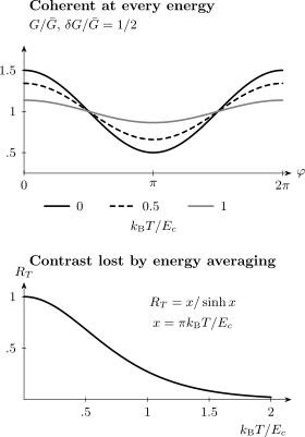
Thermal averaging of one fixed, fully coherent model. The upper curves use $\delta G/\bar G=1/2$ and temperatures $k_{\rm B}T/E_c=0,0.5,1$. The lower curve is the exact factor $x/\sinh x$. This is a calculable counterexample to identifying contrast loss with dephasing, not a universal temperature law for every interferometer.

The characteristic thermal time $\hbar/(k_{\rm B}T)$ motivates a thermal length. With explicit conventions,

$$L_T^{\rm bal}=\frac{\hbar v_F}{k_{\rm B}T},$$ $$L_T^{\rm diff}=\sqrt{\frac{\hbar D}{k_{\rm B}T}}.$$

Other correlation functions introduce factors such as $\pi$. These lengths describe energy averaging over propagation times; they are not additional measurements of the intrinsic coherence length.

Traversal, escape and level resolution

For a ballistic segment, the traversal scale is $L/v_F$. For diffusion, define

$$\tau_D=L^2/D,\qquad E_{\rm Th}=\hbar/\tau_D.$$

The Thouless energy $E_{\rm Th}$ estimates a spectral or transport correlation scale associated with exploration of that length. An exact escape time depends on boundaries and injection position; it is not universally $\tau_D$. A ring harmonic, an open cavity and a wire between absorbing contacts can weight different paths.

For a closed coherent region with mean level spacing $\delta$, the Heisenberg time is $h/\delta$. The ratio $E_{\rm Th}/\delta$ is a dimensionless measure of spectral sensitivity, related to conductance in a diffusive metal up to geometry, degeneracy and convention dependent factors. It is not an exact general identity for every device.

A small island can have a long residence time

Weak contacts let an electron remain on an island much longer than a single ballistic flight. For an isolated, noninteracting resonance with a wide-band escape width $\Gamma$, a pole at $E_0-i\Gamma/2$ gives

$$|a(t)|^2=e^{-\Gamma t/\hbar},$$ $$\tau_{\rm escape}=\hbar/\Gamma.$$

Here $\Gamma$ is the spectral full width at half maximum and the probability lifetime is $\tau_{\rm escape}$; the amplitude decays at half that rate. Extra broadening and overlapping resonances require more care.

For two contacts, $\Gamma=\Gamma_L+\Gamma_R$. The resonance transmission is

$$\mathcal T(E)=\frac{\Gamma_L\Gamma_R} {(E-E_0)^2+(\Gamma/2)^2}.$$

A symmetric contact pair reaches unit transmission at resonance. At the same total width, strongly asymmetric contacts can have a low peak. Thus the lifetime does not determine the conductance by itself. Quantum Dots develops discrete spectra and Coulomb Blockade adds charging constraints.

Terminal conductance includes the contacts

For coherent elastic normal-electron transport, count every spin and valley channel explicitly. The Landauer current is

$$I=\frac{e}{h}\int dE\,\mathcal T_{\rm tot}(E)\Delta f(E),$$

where $\Delta f=f_L-f_R$ and $\mathcal T_{\rm tot}=\sum_n\mathcal T_n$. At zero temperature and small bias,

$$G=\frac{e^2}{h}\sum_n\mathcal T_n(E_F).$$

A perfectly transmitted spin-resolved channel therefore has two-terminal resistance $h/e^2$. This does not imply dissipative scattering within that channel. In the ideal model, outgoing particles equilibrate in the macroscopic reservoirs. The central elastic scattering matrix can remain unitary even though the reservoir measurement is irreversible (Landauer; Büttiker).

Voltage probes and side contacts change which potentials and currents are compared. In linear response, microreversibility gives two-terminal $G(B)=G(-B)$ when other time-reversal-odd parameters, such as magnetization, are reversed consistently. Multiterminal reciprocity exchanges current and voltage probe pairs; it does not require each transmission coefficient to be even in field. Landauer–Büttiker Formalism develops the complete terminal construction.

Recognizing a mesoscopic signal

A static disordered sample can produce a complicated but repeatable conductance pattern as field or gate voltage is swept. Different disorder configurations produce different patterns. In a coherent metallic diffusive regime, conductance fluctuations have a characteristic root-mean-square scale of order $e^2/h$, with symmetry, geometry, degeneracy, contact and averaging factors (Altshuler; Lee and Stone). “Universal” concerns that statistical scale, not the precise trace. Universal Conductance Fluctuations explains the correlation tests.

In a ring, paths enclosing flux acquire a relative electromagnetic phase. The single-electron flux quantum is $h/e$, so an effective area $A$ gives a field period $(h/e)/A$. Harmonics, time-reversed paths and several effective areas complicate real traces; Aharonov–Bohm Rings connects these possibilities to measured oscillations. Thermal averaging and dephasing can suppress the same feature through different mechanisms.

A useful interpretation therefore combines geometry, energy resolution and controlled variation. Check repeatability, determine electronic rather than merely lithographic dimensions, and compare temperature and bias dependence with the relevant energy and path scales. A tiny sample, high mobility, low current or one conductance period is not sufficient on its own.

Exercises

1. A narrow wire needs one more comparison

A hard-wall strip has $W=70\,\mathrm{nm}$, $\lambda_F=60\,\mathrm{nm}$, $L=1.2\,\mu\mathrm m$, $\ell_{\rm tr}=0.25\,\mu\mathrm m$ and $L_\phi=4.0\,\mu\mathrm m$. Count orbital modes. Do these data establish a coherent metallic diffusive wire?

Solution

The mode count is $\lfloor2W/\lambda_F\rfloor=2$, before spin or valley factors. The sample is longer than the momentum-relaxation scale and shorter than the quoted coherence scale, but its localization length is unspecified. A two-orbital-mode wire need not have a broad metallic diffusive interval. One must check $L\ll\xi_{\rm loc}$ and the validity of the coherence model; linewidths and contacts are also needed to predict resolved plateaus. Calling the wire “diffusive” from $L>\ell_{\rm tr}$ alone would omit a crucial comparison.

2. Many collisions, little deflection

For the angular-jump model with $\theta_0=0.10$, find the probability of no collisions after time $t=20/\gamma$. Find the average projection of the final velocity onto its initial direction.

Solution

The collision number is Poisson with mean $\gamma t=20$, so the collision-free probability is $e^{-20}\simeq2.06\times10^{-9}$. After exactly $n$ independent symmetric jumps, the average cosine is $(\cos\theta_0)^n$. Summing over the Poisson distribution gives

$$\langle\cos\theta(t)\rangle =e^{-\gamma t(1-\cos\theta_0)}.$$

At the stated time this is about $0.905$. Numerous forward scattering events and weak momentum relaxation are consistent, while “collision-free” would be incorrect.

3. Thermal suppression without phase relaxation

For the cosine conductance model, derive the coefficient multiplying $\cos\varphi$ from the Fermi-weight convolution. You may use

$$\begin{aligned} F(q)&=\int_{-\infty}^{\infty}du\, \operatorname{sech}^2u\,e^{iqu},\\ F(q)&=\frac{\pi q}{\sinh(\pi q/2)}. \end{aligned}$$

Check the zero-temperature limit and the large-temperature asymptotic form.

Solution

Put $u=(E-\mu)/(2k_{\rm B}T)$ and $q=2k_{\rm B}T/E_c$. The normalized weight supplies a factor $1/2$. Its odd sine moment vanishes, leaving

$$R_T=\frac{x}{\sinh x},\qquad x=\pi k_{\rm B}T/E_c.$$

As $x\to0$, $R_T=1-x^2/6+O(x^4)$. For $x\gg1$, $R_T\simeq2xe^{-x}$. The model loses contrast through cancellation between coherent contributions at different energies; it does not contain a finite $\tau_\phi$.

4. Identical lifetimes, different resonance heights

Two isolated resonances have total width $\Gamma=10\,\mu\mathrm{eV}$. One has equal left and right widths; the other has $\Gamma_L=9.9\,\mu\mathrm{eV}$ and $\Gamma_R=0.1\,\mu\mathrm{eV}$. Compare their escape lifetimes and zero-temperature peak transmissions.

Solution

Both have $\tau_{\rm escape}=\hbar/\Gamma\simeq65.8\,\mathrm{ps}$. At resonance,

$$\mathcal T(E_0)=\frac{4\Gamma_L\Gamma_R}{\Gamma^2}.$$

The symmetric device reaches one; the asymmetric device reaches $0.0396$. Escape is set by the sum of couplings, while transmission requires entry and exit through different contacts. Finite temperature further averages the resonance, and charging or inelastic processes lie outside this model.

5. A ring can be coherent and thermally averaged

Consider a planar ring of circumference $P=4.0\,\mu\mathrm m$ and effective area $A=1.0\,\mu\mathrm m^2$, with $D=0.030\,\mathrm{m^2/s}$ and $L_\phi=6.0\,\mu\mathrm m$. Assume many channels, weak enough disorder for metallic diffusion, and $\ell_{\rm tr}\ll P$. At $T=0.10\,\mathrm K$, estimate $E_{\rm Th}=\hbar D/P^2$, $L_T$ and the $h/e$ field period. Check that the stated geometry is possible.

Solution

The estimates are

$$\begin{aligned} E_{\rm Th}&\simeq1.23\,\mu\mathrm{eV},\\ k_{\rm B}T&\simeq8.62\,\mu\mathrm{eV},\\ L_T&\simeq1.51\,\mu\mathrm m. \end{aligned}$$

The circumference is below $L_\phi$ while thermal energies exceed this Thouless estimate. Coherent winding and appreciable thermal averaging are therefore compatible; the actual harmonic amplitude still needs the ring’s path distribution and contacts.

The flux period is $(h/e)/A\simeq4.14\,\mathrm{mT}$. A planar simple closed path obeys $A\le P^2/(4\pi)\simeq1.27\,\mu\mathrm m^2$, so the proposed area is geometrically possible. Effective areas and path lengths should satisfy the same physical geometry before interpreting an oscillation.

References

• B. L. Altshuler, “Fluctuations in the Extrinsic Conductivity of Disordered Conductors,” JETP Letters 41, 648–651 (1985).
• C. W. J. Beenakker, “Random-Matrix Theory of Quantum Transport,” Reviews of Modern Physics 69, 731–808 (1997), doi:10.1103/RevModPhys.69.731.
• M. Büttiker, “Four-Terminal Phase-Coherent Conductance,” Physical Review Letters 57, 1761–1764 (1986), doi:10.1103/PhysRevLett.57.1761.
• R. Landauer, “Spatial Variation of Currents and Fields Due to Localized Scatterers in Metallic Conduction,” IBM Journal of Research and Development 1, 223–231 (1957), doi:10.1147/rd.13.0223.
• P. A. Lee and A. D. Stone, “Universal Conductance Fluctuations in Metals,” Physical Review Letters 55, 1622–1625 (1985), doi:10.1103/PhysRevLett.55.1622.
• D. J. Thouless, “Maximum Metallic Resistance in Thin Wires,” Physical Review Letters 39, 1167–1169 (1977), doi:10.1103/PhysRevLett.39.1167.

Further reading

• E. Akkermans and G. Montambaux, Mesoscopic Physics of Electrons and Photons, Cambridge University Press (2007), doi:10.1017/CBO9780511618833.
• S. Datta, Electronic Transport in Mesoscopic Systems, Cambridge University Press (1995), doi:10.1017/CBO9780511805776.
• Y. Imry, Introduction to Mesoscopic Physics, 2nd ed., Oxford University Press (2002), doi:10.1093/oso/9780198507383.001.0001.