Single-Electron Devices

A single-electron device detects or transfers individual electrons by controlling the charge states of a small island. A charge sensor converts a nearby electron into a measurable signal; a pump uses a timed sequence of tunneling events to move charge. These are different capabilities: a sensitive detector need not pump accurately, and an accurate pump need not resolve every event as it happens. The central questions are how large the signal is, how quickly the device responds, and how reliably each transfer occurs.

Required background. Coulomb Blockade supplies charge-state energies and tunneling thresholds. Quantum Point Contacts explains charge detection and finite response time. Mesoscopic Transport supplies rate equations and charge-counting statistics.

From one electron to a detector signal

A single-electron transistor (SET) has an island coupled to source and drain through tunnel junctions. Its current changes periodically with induced gate charge. For small-signal sensing, choose a flank of a Coulomb peak, where the slope is large. The current maximum has zero first-order slope, so it is usually a poor operating point for detecting a small charge change.

The detector does not generally receive an induced charge of one full electron. To see why, consider a detector island D and a target island T with mutual capacitance $C_m$. Their total capacitances $C_{D\Sigma}$ and $C_{T\Sigma}$ include $C_m$. With other electrode potentials fixed, the capacitance matrix is

$$\mathsf C= \begin{pmatrix} C_{D\Sigma}&-C_m\\ -C_m&C_{T\Sigma} \end{pmatrix}.$$

Use the charging-energy convention of the preceding page: $x_D=en_D-q_D$ and $x_T=en_T-q_T$, where $n_D,n_T$ count excess electrons and $q_D,q_T$ are gate-induced offsets. Completing the square in $\tfrac12\mathbf x^{\mathsf T}\mathsf C^{-1}\mathbf x$ gives

$$\begin{aligned} E&=\frac{(x_D+\lambda x_T)^2}{2C_{D,\mathrm{eff}}} +\frac{x_T^2}{2C_{T\Sigma}}, \\ \lambda&=\frac{C_m}{C_{T\Sigma}}, \\ C_{D,\mathrm{eff}}&=C_{D\Sigma}-\frac{C_m^2}{C_{T\Sigma}}. \end{aligned}$$

One extra target electron therefore shifts the detector’s effective offset by $-\lambda e$. The sign depends on the chosen offset convention; the signal magnitude is $\lambda e$. For output $y$, such as current or a reflected quadrature,

$$|\Delta y|\simeq \left|\frac{\partial y}{\partial q_D}\right|\lambda e.$$

This linear approximation requires a small shift along the local response curve. Large shifts need the full transfer curve. Coupling is reciprocal: fluctuations of detector charge also change the target’s addition energy. Increasing $C_m$ strengthens both the signal and this perturbation.

Sensitivity and averaging time

Let $\nu$ denote analysis frequency in hertz. Use a one-sided output-noise density $S_y(\nu)$, and define the equivalent input charge noise by

$$\begin{aligned} S_q(\nu)&=\frac{S_y(\nu)}{|\partial y/\partial q_D|^2},\\ q_n(\nu)&=\sqrt{S_q(\nu)}. \end{aligned}$$

The units of $q_n$ are charge per $\sqrt{\mathrm{Hz}}$. For white noise and a stationary signal already settled at its final value, rectangular averaging for time $\tau$ gives

$$\sigma_q=\frac{q_n}{\sqrt{2\tau}}, \qquad d=\frac{\lambda e}{\sigma_q}.$$

Here $d$ is the separation of the two means in units of their common standard deviation. It is not itself a fidelity. The Gaussian classification calculation converts that separation into an error probability under specified noise and prior assumptions. Target relaxation, missed short dwells and slow charge drift can invalidate the stationary white-noise estimate.

A charge step detects occupation, not spin directly. Spin readout first converts spin into a distinguishable charge outcome. Real-time occupation traces can also yield transfer statistics, as demonstrated by Gustavsson et al. (2006), but inferring a transferred electron from each step requires a known transport direction and enough temporal resolution.

RF readout: linewidth and settling are different quantities

In an RF-SET, the island is embedded in a matching resonator. A charge-dependent impedance changes the reflected carrier; this avoids the slow direct readout caused by a large SET resistance and stray capacitance (Schoelkopf et al., 1998).

For a linear resonator with carrier frequency $f_0$ and loaded quality factor $Q_L$, define its energy decay rate $\kappa$. Near resonance,

$$\begin{aligned} \kappa&=\frac{2\pi f_0}{Q_L},\\ \Delta f_{\mathrm{power}}&=\frac{\kappa}{2\pi} =\frac{f_0}{Q_L},\\ \tau_A&=\frac{2}{\kappa}=\frac{Q_L}{\pi f_0}. \end{aligned}$$

$\Delta f_{\mathrm{power}}$ is the full width at half maximum of the resonator’s power response. $\tau_A$ is the amplitude-envelope time constant: a small step has the normalized response $1-e^{-t/\tau_A}$. Thus a linewidth is not a complete statement of time resolution. Demodulation filters, amplifier noise and the SET’s own dynamics can impose further limits; the response to a sudden charge jump must be included in the signal model.

Loading and unloading an electron

A pump transfers charge by a periodic control sequence, potentially at zero average source–drain bias. A turnstile usually uses bias to select a direction while gates allow loading and unloading in order. The names overlap in practice; the allowed transitions define the protocol (Pekola et al., 2013).

Consider a deliberately simple model with only empty and occupied island states. During loading, the sole allowed transition is $0\to1$ from the source. During unloading, it is $1\to0$ into the drain. Let

$$\begin{aligned} a&=\exp\!\left[-\int_L\Gamma_L(t)\,dt\right],\\ b&=\exp\!\left[-\int_U\Gamma_U(t)\,dt\right]. \end{aligned}$$

$a$ is the probability that an initially empty island stays empty during loading; $b$ is the probability that an initially occupied island stays occupied during unloading. The exponentials follow from the survival equation $\dot P=-\Gamma P$. They assume a memoryless tunneling rate within each stage.

Let $p$ be the occupation probability at the beginning of loading. At the end of loading it is $p_L=1-a(1-p)$; after unloading it is $p'=bp_L$. Repeated cycles approach $p'=p$, giving

$$\begin{aligned} p&=\frac{b(1-a)}{1-ab},\\ m\equiv\langle N\rangle &=(1-b)p_L =\frac{(1-a)(1-b)}{1-ab}. \end{aligned}$$

$N$ counts electrons delivered to the drain in one cycle. Assume $ab<1$, so this periodic stationary state is reached. A failed unloading leaves charge for the next cycle. Simply multiplying the two success probabilities would describe a different protocol that resets the island to empty after every attempt, with any reset transfers counted separately.

For equal rates $\Gamma$ and equal half-period windows at drive frequency $f$,

$$\begin{aligned} a=b&=e^{-\Gamma/(2f)},\\ m&=\tanh\!\left(\frac{\Gamma}{4f}\right). \end{aligned}$$

The positive pump-current magnitude is $I=efm$; conventional current points opposite to electron motion. In the slow-drive limit the transferred count approaches one, while the current itself tends to zero because there are fewer cycles per second. At large $f/\Gamma$, this idealized model has $I\to e\Gamma/4$, well below $ef$.

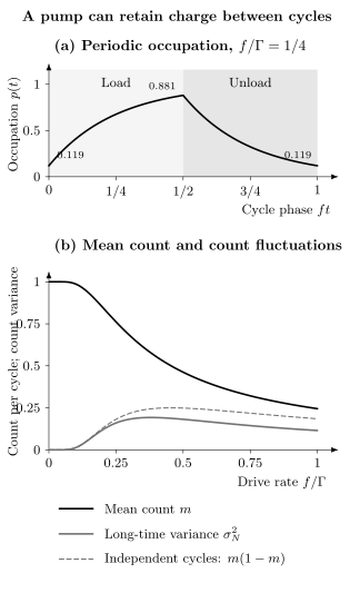
Calculated two-stage pump with unidirectional tunneling and at most one electron on the island. Top: at $f/\Gamma=1/4$, loading raises the occupation from $0.119$ to $0.881$; unloading returns it to $0.119$, so $m=0.762$ electron per cycle. Bottom: faster driving reduces $m$. The long-time count variance $\sigma_N^2$ differs from the independent-cycle estimate $m(1-m)$ because retained charge correlates successive cycles. These curves illustrate finite tunneling time; they exclude leakage, backtunneling and excited states.

Processes omitted from the two-stage model

Charging and orbital excitation energies must suppress unwanted states, while the desired rate must be fast enough during each open window. Real devices can also leak, thermally activate, tunnel back to the source or undergo virtual cotunneling. Driving more slowly suppresses missed loading but increases exposure to a roughly time-independent error rate: a small unwanted-event probability scales as $\Gamma_{\mathrm{err}}/f$. Consequently the best frequency depends on more than the desired tunneling rate (Pekola et al., 2013).

In a hybrid normal-metal–superconductor turnstile, the superconducting gap helps select single-electron events (Pekola et al., 2008). Unwanted Andreev transfer moves two electrons, and nonequilibrium quasiparticles can spoil the intended thresholds. These processes require extra transitions beyond the binary model. Integer transfer in an ordinary pump does not by itself establish a topological pumping mechanism.

What average current and noise reveal

Suppose a nominal one-electron pump delivers $N=0,1,2$ with probabilities $p_-$, $1-p_--p_+$ and $p_+$. Directly evaluating the first two moments gives

$$\begin{aligned} \langle N\rangle&=1-p_-+p_+,\\ \operatorname{Var}N&=p_-+p_+-(p_+-p_-)^2. \end{aligned}$$

The average current measures the difference of missing and extra transfers. Equal error probabilities can leave $I=ef$ even when many cycles are wrong. Noise adds information, but its interpretation also depends on correlations.

For stationary cycles, write $K_M=\sum_{k=1}^M N_k$. Define the variance accumulated per cycle over a long observation,

$$\sigma_N^2=\lim_{M\to\infty}\frac{\operatorname{Var}K_M}{M}.$$

With $C_\ell=\operatorname{Cov}(N_0,N_\ell)$ and a convergent covariance sum,

$$\sigma_N^2=\operatorname{Var}N +2\sum_{\ell=1}^{\infty}C_\ell.$$

The continuous, one-sided low-frequency noise is

$$S_I(0)=2e^2f\sigma_N^2,$$

after excluding the deterministic peaks at drive harmonics. Independent cycles give $\sigma_N^2=\operatorname{Var}N$; rare missing and extra transfers then give $S_I(0)\simeq2e^2f(p_-+p_+)$. Bursts or retained charge change that conclusion. For the two-stage model above,

$$\sigma_N^2=m-m^2\frac{1+ab}{1-ab}.$$

Exercise 3 derives this result. The figure shows why treating every cycle as a fresh Bernoulli trial overestimates its low-frequency noise. The broader relation between measured counts and current fluctuations is developed in Mesoscopic Transport; Gustavsson et al. (2006) provide an experimental example for a continuously biased quantum dot.

From a pump current to the ampere

The SI fixes $e=1.602176634\times10^{-19}\ \mathrm C$ exactly. One electron per cycle at $1\ \mathrm{GHz}$ therefore corresponds to $160.2176634\ \mathrm{pA}$. A practical current realization must still determine how many electrons actually transfer and how the measuring circuit responds (BIPM, 2019).

Observation	What it determines
Flat current versus a gate setting	Insensitivity to that setting over the measured interval
Calibrated comparison with $ef$	Mean transfer error, including current offsets and gain uncertainty
Resolved error counts	Wrong-cycle probability for the detectable event classes
Low-frequency noise	Accumulated count variance, including cycle correlations
Reversing the transfer sequence	Separates reversing pump current from nonreversing offsets

These measurements complement one another. Error counting needs a calibrated detection efficiency; a current comparison needs a calibrated current scale and enough stability during averaging. In the historical experiment of Giblin et al. (2012), the directly measured current accuracy and a smaller error inferred from a fitted pump model were explicitly different results. A fitted extrapolation does not replace a measurement at that uncertainty.

The Josephson effect and integer quantum Hall effect give another route:

$$\begin{aligned} V_J&=n_J\frac{hf_J}{2e},\\ R_H&=\frac{h}{ie^2},\\ \frac{V_J}{R_H}&=\frac{n_Ji}{2}ef_J. \end{aligned}$$

Here $n_J$ is the Josephson step index and $i$ the Hall plateau integer. Comparing this current with a pump current closes a quantum metrology triangle. Since $e$ and $h$ have exact SI values, such comparisons test practical realizations and their corrections, rather than redetermining those constants. See Fundamental Constants for the distinction between defining constants and measured quantities.

Exercises

1. How much of an electron does the sensor see?

Take $C_m=5\ \mathrm{aF}$ and $C_{T\Sigma}=100\ \mathrm{aF}$. The detector has current slope $8\ \mathrm{nA}/e$ and white one-sided output noise $20\ \mathrm{fA}/\sqrt{\mathrm{Hz}}$. Find the charge-step magnitude, input noise and ideal averaging time for $d=5$.

Solution

The coupling is $\lambda=0.05$, so the step is $0.05e$. Dividing output noise by gain gives

$$q_n=2.5\times10^{-6}\frac{e}{\sqrt{\mathrm{Hz}}}.$$

Solving the separation formula gives

$$\begin{aligned} \tau&=\frac12\left(\frac{5q_n}{0.05e}\right)^2\\ &=31.25\ \mathrm{ns}. \end{aligned}$$

This assumes a settled, stationary signal and white noise. With equal priors and equal Gaussian variances, $d=5$ gives classification error $\tfrac12\operatorname{erfc}(5/(2\sqrt2))\simeq0.00621$, not zero. Dynamics can make the error larger.

2. Can the resonator settle that quickly?

An RF sensor has $f_0=300\ \mathrm{MHz}$ and $Q_L=50$. Find its power linewidth and amplitude time constant. What fraction of a sudden signal step is reached after $31.25\ \mathrm{ns}$?

Solution

$$\begin{aligned} \Delta f_{\mathrm{power}}&=6\ \mathrm{MHz},\\ \tau_A&=\frac{50}{\pi(300\ \mathrm{MHz})}\\ &\simeq53.05\ \mathrm{ns}. \end{aligned}$$

The response fraction is $1-e^{-31.25/53.05}\simeq0.445$. The signal during this interval is substantially smaller than its final value. Exercise 1’s settled-signal estimate therefore cannot be applied directly to a newly arriving electron; the response and noise must be filtered and integrated together.

3. Count correlations in a repeated pump

For $a=b=0.2$, find the mean count and the long-time variance per cycle. Derive the variance using a counting parameter $\chi$: multiply every unloading transition by $e^\chi$. In the basis (empty, occupied), the one-cycle matrix is

$$P_\chi= \begin{pmatrix} 1&(1-b)e^\chi\\0&b \end{pmatrix} \begin{pmatrix} a&0\\1-a&1 \end{pmatrix}.$$

Solution

The largest eigenvalue $\Lambda(\chi)$ controls long runs. Put $c=ab$ and $d_0=(1-a)(1-b)$. Its characteristic equation is

$$\Lambda+\frac c\Lambda=a+b+d_0e^\chi.$$

At $\chi=0$, $\Lambda=1$. Differentiating twice yields

$$\begin{aligned} \Lambda'(0)&=\frac{d_0}{1-c}=m,\\ \Lambda''(0)&=\frac{d_0-2cm^2}{1-c}. \end{aligned}$$

The first two derivatives of $\log\Lambda$ are the mean and variance per cycle in a long run. Hence

$$\begin{aligned} \sigma_N^2&=\Lambda''(0)-m^2\\ &=m-m^2\frac{1+c}{1-c}. \end{aligned}$$

For the specified rates, $m=2/3$ and $\sigma_N^2=5/27$. An independent-cycle approximation would give $m(1-m)=2/9$, which is larger. Resetting the island to empty each cycle instead gives mean $(1-a)(1-b)=0.64$ for the intended drain-unloading events; it changes the experiment.

4. An exact mean with imperfect cycles

A pump has $p_-=p_+=2\times10^{-6}$ and independent cycles. Find its mean current, wrong-cycle probability and noise.

Solution

The errors cancel in the mean, so $I=ef$. The wrong-cycle probability is $4\times10^{-6}$ and the exact count variance is also $4\times10^{-6}$. Thus

$$S_I(0)=2e^2f(4\times10^{-6}).$$

A correct mean alone does not determine the probability of a correct individual cycle. Correlated errors would require the covariance terms as well.

5. No observed errors

An error counter observes zero errors in $M=10^7$ independent cycles. Each true wrong cycle is detected with known efficiency $\eta=0.9$, with no false counts. Find a one-sided 95% upper bound on the wrong-cycle probability $p$.

Solution

The probability of zero detected errors is $(1-\eta p)^M$. Set it to $0.05$ and solve:

$$\begin{aligned} p_{95}&=\frac{1-0.05^{1/M}}{\eta}\\ &\simeq\frac{-\ln0.05}{\eta M}\\ &\simeq3.33\times10^{-7}. \end{aligned}$$

This bound covers only errors with the stated detection efficiency. Undetected event classes, uncertain efficiency or correlated bursts require a different statistical model. Zero observed errors does not mean zero error probability.

References

• Bureau International des Poids et Mesures, “Mise en pratique for the definition of the ampere and other electric units in the SI,” SI Brochure, 9th ed., Appendix 2 (2019), BIPM publication.
• S. P. Giblin, M. Kataoka, J. D. Fletcher, P. See, T. J. B. M. Janssen, J. P. Griffiths, G. A. C. Jones, I. Farrer, and D. A. Ritchie, “Towards a Quantum Representation of the Ampere Using Single Electron Pumps,” Nature Communications 3, 930 (2012), doi:10.1038/ncomms1935.
• S. Gustavsson, R. Leturcq, B. Simovič, R. Schleser, T. Ihn, P. Studerus, K. Ensslin, D. C. Driscoll, and A. C. Gossard, “Counting Statistics of Single-Electron Transport in a Quantum Dot,” Physical Review Letters 96, 076605 (2006), doi:10.1103/PhysRevLett.96.076605.
• J. P. Pekola, O.-P. Saira, V. F. Maisi, A. Kemppinen, M. Möttönen, Y. A. Pashkin, and D. V. Averin, “Single-Electron Current Sources: Toward a Refined Definition of the Ampere,” Reviews of Modern Physics 85, 1421–1472 (2013), doi:10.1103/RevModPhys.85.1421; author manuscript.
• J. P. Pekola, J. J. Vartiainen, M. Möttönen, O.-P. Saira, M. Meschke, and D. V. Averin, “Hybrid Single-Electron Transistor as a Source of Quantized Electric Current,” Nature Physics 4, 120–124 (2008), doi:10.1038/nphys808.
• R. J. Schoelkopf, P. Wahlgren, A. A. Kozhevnikov, P. Delsing, and D. E. Prober, “The Radio-Frequency Single-Electron Transistor (RF-SET): A Fast and Ultrasensitive Electrometer,” Science 280, 1238–1242 (1998), doi:10.1126/science.280.5367.1238.