Quantum Coherence in Conductors

Phase coherence in a conductor is the retention of relative phase between alternative electronic propagation amplitudes. Static impurities can scatter an electron many times while leaving a reproducible interference pattern. Environmental dynamics, energy averaging and escape can reduce a measured interference contribution, but they are different physical processes.

This page connects a specified noise model to its phase-memory function, then explains how interference measurements constrain that function. It concerns normal-conductor orbital coherence; spin-echo times and superconducting coherence lengths describe different objects.

Required background. What Is Mesoscopic Physics? supplies the device scales and separates thermal averaging from dephasing. Reflection and Transmission Coefficients supplies current-normalized amplitudes. Boltzmann Transport supplies momentum relaxation and diffusion.

Relative phase and the averaging procedure

Consider two paths traversed during the same interval $0<t'<t$. Let their fluctuating potential-energy difference be

$$\Delta U(t')=U_1(t')-U_2(t').$$

For classical scalar noise, the additional relative phase and its average are

$$\delta\phi(t)=-\frac{1}{\hbar}\int_0^t\Delta U(t')\,dt',$$ $$\mathcal C(t)=\left\langle e^{i\delta\phi(t)}\right\rangle.$$

An interference term proportional to $A_1A_2^*$ is multiplied by $\mathcal C$. Its magnitude controls visibility and its argument shifts the fringe phase. If the same potential acts identically on both alternatives, it contributes only a common phase and cancels. The relevant noise is the difference sampled by the two paths, not an arbitrary local voltage spectrum.

The brackets must have a stated meaning. Here they average environmental realizations sampled during repeated measurements. Averaging different frozen disorder configurations can also cancel interference, although each individual sample remains coherent. Likewise, the thermal convolution combines different energies; it does not establish loss of phase within one energy-resolved scattering state.

Slow fluctuations are especially sensitive to measurement duration. A potential nearly constant during one traversal can shift a fringe; if it varies between repetitions, the accumulated trace can lose contrast. Calling that change “dephasing” should specify the averaging time and protocol. A quantum environment instead requires conditional environmental evolution or an influence functional; a classical random-phase formula is an approximation, not a replacement for that quantum calculation. Environment-Induced Decoherence gives the reduced-state description.

Gaussian noise: from a correlation function to a decay

For zero-mean classical Gaussian noise, the integrated phase is Gaussian, so

$$\mathcal C(t)=e^{-F(t)},\qquad F(t)=\frac{\langle\delta\phi(t)^2\rangle}{2}.$$

If the noise is stationary, define $K(u)=\langle\Delta U(u)\Delta U(0)\rangle$. Integrating over the two traversal times gives

$$F(t)=\frac{1}{\hbar^2}\int_0^t(t-u)K(u)\,du.$$

The factor $t-u$ counts pairs of times separated by $u$. This form makes the distinction between noise amplitude and correlation time visible.

For exponential correlations,

$$K(u)=\sigma_U^2e^{-|u|/\tau_c},$$

put $s=t/\tau_c$ and $\eta=\sigma_U\tau_c/\hbar$. The exact result is

$$F(t)=\eta^2(s-1+e^{-s}).$$

At short times the potential hardly changes during the traversal:

$$F(t)\simeq\frac{\sigma_U^2t^2}{2\hbar^2} \quad(t\ll\tau_c).$$

The decay is initially Gaussian in time. At long times, many noise fluctuations accumulate and the leading growth is

$$F(t)\sim\frac{\sigma_U^2\tau_c}{\hbar^2}t \quad(t\gg\tau_c).$$

Only when the decay occurs in that long-time regime does an exponential fit give $\tau_\phi\simeq\hbar^2/(\sigma_U^2\tau_c)$. At fixed noise variance, faster fluctuations can increase this time through motional narrowing. Holding the variance fixed is essential; fixing the integrated noise power is a different comparison.

The time defined by $F(\tau_\phi)=1$ is a useful convention for this monotone model. It need not describe an entire curve, even here. In a conductor, the noise sampled along different diffusive paths can have additional spatial correlations and different time dependence.

One fluctuator can give non-Gaussian coherence

Now let the potential difference switch between $+v$ and $-v$, with rate $\gamma$ to leave either state and equal stationary probabilities. This random telegraph noise has

$$K(u)=v^2e^{-2\gamma|u|}.$$

It shares an exponential two-point correlation with the Gaussian example but has different higher moments. Let $c_\pm(t)$ be the phase-weighted probabilities conditional on the fluctuator state, and set $\omega_0=v/\hbar$. They satisfy

$$\dot c_+=(-\gamma-i\omega_0)c_++\gamma c_-,$$ $$\dot c_-=\gamma c_++(-\gamma+i\omega_0)c_-.$$

Initially $c_+=c_-=1/2$ and $\mathcal C=c_++c_-$. Eliminating the difference gives

$$\ddot{\mathcal C}+2\gamma\dot{\mathcal C} +\omega_0^2\mathcal C=0.$$

For $\omega_0>\gamma$, define $\Omega=\sqrt{\omega_0^2-\gamma^2}$. The solution is

$$\mathcal C(t)=e^{-\gamma t}Q(t),$$ $$Q(t)=\cos(\Omega t)+\frac{\gamma}{\Omega}\sin(\Omega t).$$

The coherence can cross zero and revive. A negative value means a fringe-phase shift of $\pi$; visibility is $|\mathcal C|$, never a negative intensity. The Gaussian approximation with the same $K(u)$ misses those revivals. In the rapid-switching weak-coupling limit, $\omega_0\ll\gamma$, it recovers the leading decay rate $\omega_0^2/(2\gamma)$ (Paladino and colleagues).

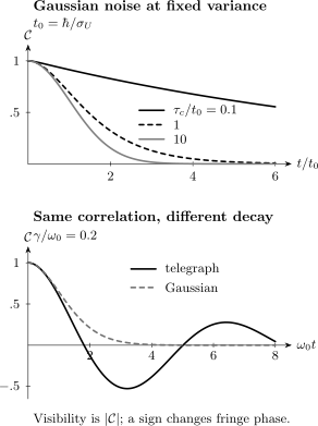
Upper panel: Gaussian noise at fixed variance, with $t_0=\hbar/\sigma_U$ and three correlation times. Rapid fluctuations produce slower long-time decay. Lower panel: telegraph noise with $\gamma/\omega_0=0.2$ and the Gaussian model with the same $K(u)$. Their different coherence functions show why a noise spectrum alone is insufficient when the noise is non-Gaussian.

A single $1/e$ crossing can be quoted for a nonmonotone curve, but it does not summarize its zeros, phase reversals or revivals. These elementary models teach how to interpret a decay; they are not universal laws for electron–electron dephasing in a metal.

Coherent diffusion and its cutoffs

For diffusion, use $L_\phi=\sqrt{D\tau_\phi}$. It is a displacement scale reached during a phase-memory time, not the total length of a scattered trajectory. In ballistic motion the corresponding convention is $v_F\tau_\phi$.

Disorder-averaged propagator pairs organize into diffusion modes. The diffuson describes probability propagation, while the Cooperon describes interference involving time-reversed paths. For one phenomenological Cooperon channel at zero magnetic field,

$$\mathcal P_{C,n}(\omega)\propto \frac{1}{Dq_n^2+\gamma_\phi+\gamma_s-i\omega}.$$

Here $\gamma_\phi=1/\tau_\phi$ and $\gamma_s$ is a specified channel relaxation rate. The allowed $q_n$ depend on boundaries. Orbital magnetic field changes the diffusion operator; spin–orbit coupling mixes singlet and triplet channels and cannot generally be represented by one extra scalar rate.

Do not add $\gamma_\phi$ indiscriminately to a conserved probability mode: loss of interference does not destroy particles. Likewise, suppressing time-reversed interference with a static magnetic field does not imply that every electronic amplitude has lost coherence. Weak Localization develops the conductivity correction and symmetry-dependent signs.

Escape can imitate lifetime saturation

An exactly solvable finite-size example is a one-dimensional interval with absorbing contacts at $x=0,L$. Its diffusion modes are $\sin(n\pi x/L)$, so the slowest phenomenological Cooperon decays at

$$\lambda_1=\frac{\pi^2D}{L^2}+\frac{1}{\tau_\phi}.$$

If this mode were incorrectly fitted as intrinsic decay alone, the inferred lifetime would approach

$$\tau_{\rm fit}\longrightarrow\frac{L^2}{\pi^2D}$$

as the true $\tau_\phi$ grows. The corresponding fitted length would approach $L/\pi$. These are results for this boundary problem, not universal saturation values. They demonstrate why escape and geometry belong in the forward model.

Independent exponential phase-noise factors multiply, so their rates add. For nonexponential factors it is the full functions $F_i(t)$ that add, when the noises are independent. Correlated mechanisms, spin-channel matrices and different spatial modes require more than a sum of fitted inverse times.

Physical sources of phase relaxation

Electron–electron interactions can conserve the total electronic energy while transferring phase information from one excitation into many others. Small-energy-transfer fluctuations in diffusive metals produce Nyquist dephasing. The Altshuler–Aronov–Khmelnitsky treatment gives representative low-temperature scales in a weakly disordered Fermi liquid:

Diffusive regime	Representative rate dependence
Quasi-one-dimensional	$\tau_\phi^{-1}\propto T^{2/3}$
Two-dimensional	$\tau_\phi^{-1}\sim(k_{\rm B}T/\hbar g_\square)\ln g_\square$
Three-dimensional, dirty small-transfer contribution	$\tau_\phi^{-1}\propto T^{3/2}$

Here $g_\square=\sigma_\square/(e^2/h)\gg1$ in the two-dimensional metallic regime. Coefficients, screening and competing large-energy-transfer contributions depend on the system. These are not arbitrary fitting exponents for localized, ballistic, strongly correlated or driven conductors. In particular, the quasi-one-dimensional result can involve nonexponential path averages; the exponent does not prove a single exponential envelope.

For interference, transverse dimensions must be below the distances explored by the relevant coherent modes. For the quoted low-temperature interaction regimes, thermal diffusion lengths also enter. Thus a geometrically narrow wire need not have one-dimensional electronic bands, and a change in temperature can change the effective dimension of its dephasing calculation.

Electron–phonon coupling, magnetic impurities, charge fluctuators and external electromagnetic fields provide other channels. Phonon powers depend on disorder and phonon confinement; magnetic moments introduce spin dynamics and Kondo crossovers; detectors can acquire which-path information. A power law over a short range rarely identifies one mechanism uniquely.

The classical Gaussian model must not be extended to equilibrium zero-point fluctuations by simply inserting a symmetrized quantum noise spectrum. Emission, absorption, recoil and Pauli blocking matter for electrons near the Fermi surface. In an equilibrium nonmagnetic diffusive Fermi liquid, standard electron–electron and electron–phonon contributions vanish toward zero temperature (Marquardt and colleagues). Finite-energy injected particles and driven environments need not obey that equilibrium limit.

How measurements constrain phase memory

Different observables weight different path families. Agreement is useful when their geometry and temperature factors have been treated consistently; disagreement can reveal an inadequate model rather than an arithmetic mistake.

Measurement	What must be modeled
Weak localization or antilocalization	Return loops, magnetic field and spin channels
Conductance fluctuations	Field/energy correlations and thermal convolution
Ring harmonics	Winding, contacts and path-duration distributions
Cavity fringes	Reflections, mode balance and energy resolution
Resonance linewidth	Escape and other broadening, not pure dephasing alone

Magnetoconductance

For one simplified two-dimensional fitting convention, define $\Delta\sigma(B)=\sigma(B)-\sigma(0)$ and

$$\Delta\sigma(B)=\alpha\frac{e^2}{2\pi^2\hbar} \mathcal F(|B|/B_\phi),$$ $$\mathcal F(z)=\psi\!\left(\frac12+\frac1z\right)+\ln z,$$ $$B_\phi=\frac{\hbar}{4eL_\phi^2}.$$

The zero-field limit is continuous: $\mathcal F(z)\sim z^2/24$. In this sign convention, positive $\alpha$ gives a positive weak-localization magnetoconductance; negative $\alpha$ gives an antilocalization cusp. Reversing the definition of $\Delta\sigma$ reverses the apparent prefactor sign. Real spin, valley and surface-channel structures require the corresponding combinations of terms (Hikami, Larkin and Nagaoka).

A fitted $\alpha$ is not automatically a channel count. Field range, classical background, interaction corrections and parameter covariance matter. The formula assumes diffusive two-dimensional transport in its applicable field range; it should not be extended through a dimensional or ballistic crossover merely because a fit remains smooth.

Fluctuation correlations and ring harmonics

A conductance-fluctuation correlation field satisfies a scale estimate $B_cA_\phi\sim h/e$. For a narrow wire the relevant area is often of order $wL_\phi$; in a two-dimensional patch it is of order $L_\phi^2$. This is not the definition of the magnetoconductance parameter $B_\phi$. Numerical coefficients and the correlation-width convention must be specified.

The intrinsic zero-temperature energy correlation is often set by $\hbar D/L_{\rm eff}^2$, with geometry, escape and phase relaxation determining the effective length. Thermal averaging can reduce variance and broaden the measured energy correlation without shortening the intrinsic $L_\phi$. Use the thermal-convolution lesson and Universal Conductance Fluctuations rather than replacing $L_\phi$ by $L_T$ automatically.

For a ring, a common phenomenological amplitude has a factor $\exp(-nP/L_\phi)$ for winding number $n$ and circumference $P$. Its remaining coefficient depends on contacts, thermal averaging and the chosen harmonic. Ratios of adjacent measured harmonics therefore do not determine $L_\phi$ unless those coefficients are controlled. Aharonov–Bohm Rings develops the appropriate path models.

Interpreting a low-temperature plateau

A plateau in a fitted lifetime is an observation to explain. Electron temperature can stop tracking the refrigerator; finite size and escape can limit the longest visible paths; weak magnetic contamination, detector bias, microwave leakage and fit resolution can matter. Controlled studies of metallic wires found that source purity and dilute magnetic impurities can account for several saturation-like behaviors (Pierre and colleagues). That result does not identify every plateau in every device.

Useful comparisons change one possible limit at a time: excitation current and detector bias, filtering, sample length, impurity content, or the field range used in the fit. Compare a second interference observable where possible. Report a lower bound when the measurement is insensitive to further increases of $\tau_\phi$ instead of interpreting the best-fit plateau as an intrinsic constant.

Finite bias is another reason for care. A wire can have a double-step distribution rather than a hotter Fermi function; energy averaging, heating and nonequilibrium scattering can coexist. One effective temperature is justified only when the distribution and relaxation support it.

Finally, orbital $L_\phi$ is not a spin relaxation length, spin-echo $T_2$, inhomogeneous $T_2^*$ or superconducting pair coherence length. Decoherence Timescales and Spin Qubits explain the distinct protocols.

Exercises

1. Which potential fluctuations matter?

For equal traversal intervals, suppose $U_1(t)=X(t)+Y_1(t)$ and $U_2(t)=X(t)+Y_2(t)$. The three zero-mean processes are independent, and the two $Y$ processes have identical covariance $K_Y(u)$. Find the covariance that enters the Gaussian relative-phase decay.

Solution

The shared $X$ cancels exactly. The difference is $Y_1-Y_2$, whose covariance is $2K_Y(u)$ because the cross correlations vanish. Thus

$$F(t)=\frac{2}{\hbar^2}\int_0^t(t-u)K_Y(u)\,du.$$

If the two paths instead sample the same $Y$, it also cancels. Noise amplitude at one point is insufficient: correlations between the alternatives matter. Unequal time intervals or spatially different coupling require the actual path-dependent difference.

2. Derive the Gaussian crossover

Integrate $K(u)=\sigma_U^2e^{-u/\tau_c}$ in the expression for $F(t)$. Explain why the long-time inverse decay rate is not valid when $\sigma_U\tau_c/\hbar\gg1$.

Solution

The elementary integral is

$$J(t)=\int_0^t(t-u)e^{-u/\tau_c}du,$$ $$J(t)=\tau_c t-\tau_c^2(1-e^{-t/\tau_c}).$$

It gives $F=\eta^2(s-1+e^{-s})$. When $\eta\gg1$, the $1/e$ decay occurs at $t\simeq\sqrt2\hbar/\sigma_U\ll\tau_c$, in the Gaussian short-time regime. Extrapolating the long-time exponential rate backward would therefore predict the wrong characteristic time.

3. Escape-limited apparent coherence

For the absorbing interval, take $L=10\,\mu\mathrm m$, $D=0.020\,\mathrm{m^2/s}$ and intrinsic $\tau_\phi=0.80\,\mathrm{ns}$. Find $1/\lambda_1$ and the length obtained by mistakenly treating it as the intrinsic phase time. What happens as the true lifetime diverges?

Solution

The intrinsic length is $4.0\,\mu\mathrm m$. Escape alone has time $L^2/(\pi^2D)\simeq0.507\,\mathrm{ns}$. Adding the two mode rates gives

$$1/\lambda_1\simeq0.310\,\mathrm{ns},$$

and the mistaken length is $\sqrt{D/\lambda_1}\simeq2.49\,\mu\mathrm m$. With vanishing intrinsic rate, these approach $0.507\,\mathrm{ns}$ and $L/\pi\simeq3.18\,\mu\mathrm m$. The apparent plateau is entirely a finite-boundary effect in this example.

4. Same correlation, different coherence

Let telegraph switching become arbitrarily slow while the initial fluctuator state remains equally likely to be $+v$ or $-v$. Find $\mathcal C(t)$ and compare with a Gaussian static offset of variance $v^2$.

Solution

The two phases are $\pm vt/\hbar$, so

$$\mathcal C_{\rm telegraph}(t)=\cos(vt/\hbar).$$

The Gaussian average is

$$\mathcal C_{\rm Gaussian}(t)=e^{-v^2t^2/(2\hbar^2)}.$$

Both offsets have zero mean and the same constant two-point correlation, but their distributions differ. The telegraph average revives; the Gaussian one does not. Within an individual run with a fixed offset there is a deterministic phase, so the contrast loss here refers to averaging runs with unknown offsets.

5. A harmonic ratio needs its prefactors

Assume $A_n=a_n\exp(-nP/L_\phi)$, where $a_n$ includes thermal and contact effects. A ring with $P=3\,\mu\mathrm m$ has $A_2/A_1=0.10$. Compare the inferred length for $a_2/a_1=1$ and $1/2$.

Solution

For equal prefactors, $e^{-P/L_\phi}=0.10$, giving $L_\phi=P/\ln10\simeq1.30\,\mu\mathrm m$. For ratio $1/2$, the exponential is $0.20$, giving $L_\phi=P/\ln5\simeq1.86\,\mu\mathrm m$.

The same measured ratio supports different lengths when the prefactor is unknown. Harmonic amplitudes constrain a model; they do not eliminate its thermal and contact assumptions.

References

• B. L. Altshuler, A. G. Aronov, and D. E. Khmelnitsky, “Effects of Electron–Electron Collisions with Small Energy Transfers on Quantum Localisation,” Journal of Physics C: Solid State Physics 15, 7367–7386 (1982), doi:10.1088/0022-3719/15/36/018.
• S. Hikami, A. I. Larkin, and Y. Nagaoka, “Spin–Orbit Interaction and Magnetoresistance in the Two-Dimensional Random System,” Progress of Theoretical Physics 63, 707–710 (1980), doi:10.1143/PTP.63.707.
• F. Marquardt, J. von Delft, R. A. Smith, and V. Ambegaokar, “Decoherence in Weak Localization. I. Pauli Principle in Influence Functional,” Physical Review B 76, 195331 (2007), doi:10.1103/PhysRevB.76.195331.
• E. Paladino, Y. M. Galperin, G. Falci, and B. L. Altshuler, “1/f Noise: Implications for Solid-State Quantum Information,” Reviews of Modern Physics 86, 361–418 (2014), doi:10.1103/RevModPhys.86.361.
• F. Pierre, A. B. Gougam, A. Anthore, H. Pothier, D. Esteve, and N. O. Birge, “Dephasing of Electrons in Mesoscopic Metal Wires,” Physical Review B 68, 085413 (2003), doi:10.1103/PhysRevB.68.085413.

Further reading

• E. Akkermans and G. Montambaux, Mesoscopic Physics of Electrons and Photons, Cambridge University Press (2007), doi:10.1017/CBO9780511618833.
• J. J. Lin and J. P. Bird, “Recent Experimental Studies of Electron Dephasing in Metal and Semiconductor Mesoscopic Structures,” Journal of Physics: Condensed Matter 14, R501–R596 (2002), doi:10.1088/0953-8984/14/18/201.