Quantum Point Contacts

A quantum point contact (QPC) is a tunable bottleneck that connects two electron reservoirs through a few transverse modes. Raising its electrostatic barrier closes those modes one by one. The same sensitivity makes a QPC a charge detector: an electron added to a nearby dot shifts the barrier and changes the QPC current.

We study a clean semiconductor constriction and then its detector operation. The short elastic scattering region is distinct from the reservoirs, where outgoing carriers relax. Conductance Quantization derives the channel-current and noise formulas used here; Quantum Dots explains the target’s addition spectrum.

Required background. Two-Dimensional Electron Gases supplies the reservoir density and confinement, Quantum Wires supplies transverse modes, and Reflection and Transmission Coefficients supplies probabilities normalized to current.

Gates create an electronic bottleneck

In a split-gate device, negative surface-gate voltages deplete the electron gas below them and narrow the remaining conducting path. Fringing fields, screening and the depth of the 2DEG determine the electronic width; it is generally smaller than the lithographic opening and changes with voltage. Electrostatic modeling must include the exposed surface and dielectric geometry (Davies, Larkin and Sukhorukov, 1995).

Changing both gates together mainly shifts the barrier and confinement. Changing their difference moves the channel sideways and changes its shape, which helps distinguish a clean bottleneck from a nearby defect. Neither operation is an exactly pure control knob: both can also shift a neighboring dot or its tunnel barriers.

A useful few-mode regime has electronic width comparable to the local Fermi wavelength and constriction length $L_c$ much shorter than the elastic mean free path. A coherent scattering description also requires negligible phase randomization during passage. It does not require a phase-coherent macroscopic circuit.

For a spin-degenerate, single-valley reservoir,

$$\lambda_F=\sqrt{\frac{2\pi}{n_{2\mathrm D}}}.$$

The density $2.0\times10^{15}\,\mathrm m^{-2}$ gives $\lambda_F\simeq56\,\mathrm{nm}$. An undepleted hard-wall opening of width $W$ would have roughly $2W/\lambda_F$ orbital modes. This is a scale estimate: the reservoir density is not the depleted bottleneck density, and a longitudinal barrier can close a mode that would fit geometrically.

To resolve adjacent zero-bias steps, their spacing must exceed thermal rounding, intrinsic transmission rounding and relevant disorder broadening. A short ballistic device can therefore have poorly resolved steps. Conversely, narrow peaks or closed charging diamonds may indicate an unintended island; use Coulomb Blockade to interpret that regime.

Local modes can reflect without mixing

At each longitudinal position $x$, solve the transverse problem in $y$:

$$H_\perp(x)\phi_n(y;x)=\varepsilon_n(x)\phi_n(y;x).$$

Expanding $\Psi=\sum_n\chi_n(x)\phi_n(y;x)$ turns the two-dimensional problem into coupled longitudinal channels. Spatial derivatives of the transverse states produce couplings

$$P_{mn}=\langle\phi_m|\partial_x\phi_n\rangle.$$

A useful test away from degeneracies is

$$\hbar|v_xP_{mn}|\ll|\varepsilon_m-\varepsilon_n|,$$

for $m\ne n$, together with control of second-derivative terms. Parity can suppress some couplings; an asymmetric gate can restore them. A small longitudinal velocity does not by itself validate this test at a turning point.

Even when transitions between modes are negligible, the diagonal projection contains a geometric correction. For a real normalized mode on an interval without a degeneracy,

$$U_n^{\rm eff}=\varepsilon_n+\Phi_n,$$ $$\Phi_n=\frac{\hbar^2}{2m^*} \langle\partial_x\phi_n|\partial_x\phi_n\rangle\ge0.$$

For a general complex basis, the connection and orthogonal projection must be retained together; Quantum Wires gives that derivation. Dropping $\Phi_n$ is an additional approximation. The maximum of the resulting effective potential can reflect a particle in the same mode. Adiabatic mode propagation and perfect transmission are different statements.

The saddle model

Near a smooth bottleneck, approximate the potential by

$$U(x,y)=U_0-\frac{m^*\omega_x^2x^2}{2} +\frac{m^*\omega_y^2y^2}{2}.$$

The transverse oscillator is independent of $x$ in this separable model, so its derivative couplings vanish. The threshold for orbital $n=0,1,\ldots$ is

$$E_n^{\rm top}=U_0+\hbar\omega_y(n+1/2).$$

Define the longitudinal rounding scale $s=\hbar\omega_x/(2\pi)$. The inverted-oscillator solution gives

$$T_n(E)=\frac1{1+e^{-(E-E_n^{\rm top})/s}}.$$

Thus $T_n=1/2$ at threshold, while well-separated nearly open modes require $s$ and $k_{\mathrm B}T$ small compared with $\hbar\omega_y$. A smaller longitudinal curvature makes a broader spatial barrier and a sharper energy riser. The saddle is a local approximation matched to leads, not a potential that remains an inverted parabola throughout the device (Büttiker, 1990).

Read conductance and bias maps

For twofold spin degeneracy without resolved splitting, write $G_0=2e^2/h$. At low temperature and small bias,

$$G=G_0\sum_nT_n(\mu).$$

At finite temperature, average each transmission with $-\partial_E f$. Plateaus then describe nearly binary transmissions, not integer charge trapped inside the QPC. Conductance alone measures their sum; partition noise constrains a different combination, $\sum_aT_a(1-T_a)$, where $a$ counts resolved internal channels.

In the low-temperature shot-noise regime with energy-independent transmissions,

$$S_I^{(1)}=2e|I|F,$$ $$F=\frac{\sum_aT_a(1-T_a)}{\sum_aT_a}.$$

Here the low-frequency spectral density is one-sided in ordinary frequency. The partition term vanishes for perfect channels, but equilibrium thermal noise and amplifier noise remain. The finite-temperature crossover is derived in Conductance Quantization.

A threshold line measures relative motion

Let a local gate change be $\delta V_g$, and model the barrier response as

$$E_n^{\rm top}=E_n^0-\alpha e\delta V_g+\beta eV.$$

Choose source and drain potentials

$$\mu_S=\mu_0+\eta eV,$$ $$\mu_D=\mu_0-(1-\eta)eV.$$

The positive lever arm $\alpha$, bias division $\eta$ and barrier shift $\beta$ are local model parameters. Alignment with source or drain produces transconductance ridges. Their slopes satisfy

$$\alpha\frac{dV_g}{dV}=\beta-\eta \quad\text{(source)},$$ $$\alpha\frac{dV_g}{dV}=\beta+1-\eta \quad\text{(drain)}.$$

The ridge positions therefore do not determine a lever arm without assumptions about electrostatics. For a rigid saddle and symmetric bias, the slopes are opposite and a threshold inside the bias window contributes a half-step to differential conductance. Barrier motion, asymmetric voltage division, heating or interactions change that conclusion. Finite-bias gate maps are not universal diamond templates.

An interaction-related shoulder near $0.7G_0$, resonances and series resistance can distort the simple staircase. Conductance Quantization discusses these alternatives. Independently calibrate series resistance rather than choosing it solely to align plateaus.

Turn a barrier shift into a charge signal

A capacitively coupled dot changes the QPC potential without sending its electron through the detector. This permits charge sensing even when direct dot current is too small to measure (Field and colleagues, 1993). For a small effective gate shift $\delta V_g$ at detector bias $V_d$,

$$\Delta I\simeq V_d\frac{\partial G}{\partial V_g}\delta V_g.$$

Equivalently, on one saddle riser a small threshold shift $\delta E$ produces

$$\delta T\simeq-\frac{T(1-T)}s\delta E.$$

A plateau is quiet in partition noise but insensitive to a barrier shift. The slope is largest at $T=1/2$. In the ideal shot-noise-dominated, fixed-coupling limit, signal squared divided by noise is also proportional to $T(1-T)$. This does not establish a universal best operating point: gate-dependent coupling, amplifier noise, additional channels and disturbance of the dot all matter.

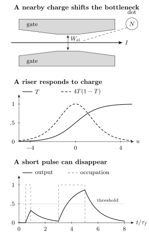
Top: a schematic conducting bottleneck and nearby target dot; dashed coupling indicates an electrostatic interaction, not particle exchange. Middle: calculated saddle transmission $T$ and normalized small-shift response $4T(1-T)$ against $u=(\mu-E^{\rm top})/s$. Bottom: an ideal first-order detector filters two unit-height charge pulses of durations $0.4\tau_f$ and $2\tau_f$. The short pulse never reaches the half-height threshold. These illustrative curves use the models in the text, not experimental data.

Sensitivity, averaging and classification

Let $\mathcal R_q=|\partial I/\partial q|$. The input-referred charge sensitivity is $\sqrt{S_I^{(1)}}/\mathcal R_q$, in $\mathrm C/\sqrt{\mathrm{Hz}}$. For white current noise and a rectangular average of duration $\tau$,

$$\sigma_{\bar I}^2=\frac{S_I^{(1)}}{2\tau}.$$

Define the separation in units of the standard deviation of one state as $d=|\Delta I|/\sigma_{\bar I}$. Then

$$d^2=\frac{2(\Delta I)^2\tau}{S_I^{(1)}}.$$

For equal priors and two stationary Gaussian distributions of equal variance, a midpoint threshold gives

$$P_{\rm err}=\frac12\operatorname{erfc} \left(\frac{d}{2\sqrt2}\right).$$

Thus $d=5$ gives about $0.62\%$ classification error, not a five-standard-deviation tail: the decision boundary is only $d/2$ from either mean. Different definitions of signal-to-noise ratio produce different numerical factors. State changes during the integration window and unequal noise require a different classifier (Clerk and colleagues, 2010).

A fast sample rate does not recover a filtered event

For an ideal first-order filter with time constant $\tau_f$, normalized output $y$ obeys

$$\tau_f\dot y+y=n(t),$$

where $n(t)$ is the dot occupation change. A pulse lasting $t_d$ reaches only $1-e^{-t_d/\tau_f}$. A half-height threshold misses an isolated pulse when

$$t_d<\tau_f\ln2.$$

This simple calculation explains the missed-event problem. Real tunneling traces contain successive stochastic pulses, so one must fit the detector response and transition process together; merely discarding short intervals does not reconstruct the underlying rates (Naaman and Aumentado, 2006). A higher sampling rate helps describe the filtered trace but cannot undo information lost below its noise floor.

Radio-frequency readout can raise bandwidth and reduce sensitivity to low-frequency drift by embedding the QPC in a resonator. The resonator response, amplifier noise and digital filtering then all enter the event resolution.

The detector also changes the target

Static capacitive shifts, heating and emission of electrical or phonon excitations can alter dot levels and tunneling. Raising detector bias may increase the signal while making those effects worse. Target excitation rates depend on frequency-resolved noise, not just the measured low-frequency current-noise level.

Measurement itself also reduces coherence. For target charge state $j$, one scattered detector electron leaves in

$$|D_j\rangle=r_j|L\rangle+t_j|R\rangle.$$

Tracing out that electron multiplies the target off-diagonal density-matrix element by

$$\nu=\langle D_1|D_0\rangle =r_1^*r_0+t_1^*t_0.$$

After $M$ independent identical scattering events, its magnitude is multiplied by $|\nu|^M$. This model assumes the target charge is conserved during each event and does not describe heating-induced transitions. A current record senses transmission probabilities; target-dependent relative scattering phases can reduce $|\nu|$ even when those probabilities are identical (Averin and Sukhorukov, 2005). The which-path experiment of Buks and colleagues (1998) illustrates the connection between detector coupling and lost interference.

A QPC detects spin through spin-to-charge conversion. Energy-selective tunneling or Pauli blockade first makes charge motion depend on spin; the QPC reads the resulting charge history (Elzerman and colleagues, 2004). Detector classification error is only one contribution to total readout error; conversion failure and relaxation also matter. See Spin Qubits.

Observation	Useful comparison
Conductance riser	Temperature and bias dependence
Nearly integer plateau	Partition noise and independent series resistance
Narrow resonance	Lateral gate shift and charging spectroscopy
Charge step	Target-gate dependence versus trap switching
Apparent tunnel rate	Detector response and missed pulses
Faster readout at larger bias	Target rates, heating and relaxation

In a quantum Hall device a partly transmitting QPC also acts as a beam splitter for edge channels. Its terminal geometry must respect chirality; Integer Quantum Hall Effect explains that setting.

Exercises

1. Separate shape change from reflection. In a separable saddle, do vanishing transverse derivative couplings imply $T=1$? Evaluate $T$ when $\hbar\omega_x=0.40\,\mathrm{meV}$ and $E-E^{\rm top}=0.20\,\mathrm{meV}$.

Solution

No. The transverse oscillator basis is fixed, but each channel still crosses an inverted longitudinal oscillator. The transmission is $T=(1+e^{-\pi})^{-1}\simeq0.959$; at threshold it is $1/2$. Mode conservation does not forbid same-mode reflection.

2. Interpret two ridge slopes. A local model has $\alpha=0.10$, $\eta=1/2$ and $\beta=0.20$. Find the source and drain slopes $dV_g/dV$. Can the midpoint displacement be attributed uniquely to asymmetric reservoir bias?

Solution

The slopes are $-3$ and $+7$. Their difference is $1/\alpha=10$, while their mean is $2$. The asymmetry here comes entirely from barrier motion. More generally the mean constrains $(\beta+1/2-\eta)/\alpha$, not $\eta$ alone. Extracting a spacing also assumes neighboring thresholds share the modeled response.

3. Translate sensitivity into error. A one-electron signal is $100\,\mathrm{fA}$ and the one-sided white-noise amplitude is $20\,\mathrm{fA}/\sqrt{\mathrm{Hz}}$. Find the averaging time for $d=5$ and the equal-prior Gaussian error.

Solution

From the specified definition,

$$\tau=\frac{25S_I^{(1)}}{2(\Delta I)^2} =0.50\,\mathrm s.$$

The midpoint lies $2.5$ standard deviations from each mean, giving $P_{\rm err}\simeq0.00621$. This slow illustrative detector cannot resolve a target that switches much faster than the integration time. White stationary noise and a constant target state were essential assumptions.

4. Find a missed pulse. A first-order detector has $\tau_f=10\,\mu\mathrm s$. Compare isolated occupation pulses lasting $4\,\mu\mathrm s$ and $20\,\mu\mathrm s$ at a half-height threshold.

Solution

Their peak outputs are $1-e^{-0.4}=0.330$ and $1-e^{-2}=0.865$. Only the second crosses $1/2$. The minimum duration is $\tau_f\ln2=6.93\,\mu\mathrm s$. Even noiseless sampling at a much higher rate does not make a half-height classifier detect the first pulse; a different inference model would need its shape and noise level.

5. Dephase without a current contrast. Let

$$|D_0\rangle=\frac{|L\rangle+|R\rangle}{\sqrt2},$$ $$|D_1\rangle=\frac{|L\rangle+e^{i\theta}|R\rangle}{\sqrt2}.$$

Compare charge-counting probabilities and target coherence after $M$ electrons.

Solution

Both states transmit with probability $1/2$, so the entire count distribution is identical for the two target charges. Nevertheless,

$$|\nu|=|\cos(\theta/2)|.$$

The coherence magnitude is reduced by $|\cos(\theta/2)|^M$. For $\theta=\pi/2$ and $M=10$, the factor is $1/32$. The outgoing phase contains information unavailable to a simple transmitted-current measurement; an interferometric measurement can in principle access it.

References

• D. V. Averin and E. V. Sukhorukov, “Counting Statistics and Detector Properties of Quantum Point Contacts,” Physical Review Letters 95, 126803 (2005), doi:10.1103/PhysRevLett.95.126803, arXiv:cond-mat/0505647.
• E. Buks, R. Schuster, M. Heiblum, D. Mahalu and V. Umansky, “Dephasing in Electron Interference by a ‘Which-Path’ Detector,” Nature 391, 871–874 (1998), doi:10.1038/36057.
• M. Büttiker, “Quantized Transmission of a Saddle-Point Constriction,” Physical Review B 41, 7906–7909 (1990), doi:10.1103/PhysRevB.41.7906.
• A. A. Clerk, M. H. Devoret, S. M. Girvin, F. Marquardt and R. J. Schoelkopf, “Introduction to Quantum Noise, Measurement, and Amplification,” Reviews of Modern Physics 82, 1155–1208 (2010), doi:10.1103/RevModPhys.82.1155, author-hosted paper.
• J. H. Davies, I. A. Larkin and E. V. Sukhorukov, “Modeling the Patterned Two-Dimensional Electron Gas: Electrostatics,” Journal of Applied Physics 77, 4504–4512 (1995), doi:10.1063/1.359446.
• J. M. Elzerman, R. Hanson, L. H. Willems van Beveren, B. Witkamp, L. M. K. Vandersypen and L. P. Kouwenhoven, “Single-Shot Read-Out of an Individual Electron Spin in a Quantum Dot,” Nature 430, 431–435 (2004), doi:10.1038/nature02693, arXiv:cond-mat/0411232.
• M. Field, C. G. Smith, M. Pepper, D. A. Ritchie, J. E. F. Frost, G. A. C. Jones and D. G. Hasko, “Measurements of Coulomb Blockade with a Noninvasive Voltage Probe,” Physical Review Letters 70, 1311–1314 (1993), doi:10.1103/PhysRevLett.70.1311.
• O. Naaman and J. Aumentado, “Poisson Transition Rates from Time-Domain Measurements with a Finite Bandwidth,” Physical Review Letters 96, 100201 (2006), doi:10.1103/PhysRevLett.96.100201.