Nanostructures for Quantum Technology

A nanostructure can store a spin, detect one electron, transfer a known charge or host a superconducting bound state. Making that effect useful requires a repeatable sequence of preparation, control and measurement. This page explains how to connect those operations to device parameters, using small calculations that expose the tradeoffs hidden by a single coherence time or fidelity.

Required background. What Is Mesoscopic Physics? introduces confinement, transport and coherence scales; Quantum Dots explains discrete charge and orbital states. Measurement Backaction explains why obtaining information can disturb a quantum system.

Quantum states and the operating cycle

Start with the physical degree of freedom. In a spin qubit, two spin states span the computational subspace; orbital, valley and additional charge states can provide unwanted escape routes. A current source instead aims to transfer an integer charge per cycle. Its transfer probability, rather than a qubit gate fidelity, measures the relevant success.

Device function	Physical calculation to start with
Store and rotate a spin	Splitting, driven transitions and relaxation in spin qubits
Detect an island charge	Signal contrast, noise and response time in quantum point contacts
Transfer a known charge	Loading and escape probabilities in single-electron devices
Control a superconducting bound state	Occupations, parity and transition energies in Andreev physics

For a driven two-level system, choose a frame rotating at the drive frequency. After the rotating-wave approximation, a useful Hamiltonian is

$$H_{\mathrm{rot}}(t)=\frac{\hbar}{2} \left[\delta(t)\sigma_z+\Omega(t)\sigma_x\right].$$

Here $\delta$ is angular-frequency detuning and $\Omega$ is the resonant Rabi frequency for a drive of fixed phase. On resonance, a constant pulse rotates by $\Omega\tau$. Thus a larger drive shortens a rotation, but it also changes coupling to nearby transitions. A pulse envelope of duration $\tau$ has a spectral width of order $1/\tau$; its precise tails depend on its shape. Leakage depends on those tails and the transition matrix elements. Comparing $\hbar/\tau$ with an energy separation is a useful first check, not a calculation of leakage probability.

For two electron spins, electrically controlled exchange gives $H_{\mathrm{ex}}=J(t)\mathbf s_1\cdot\mathbf s_2$, with $\mathbf s=\boldsymbol\sigma/2$. The singlet–triplet energy difference is $J$, so the relative phase is $\hbar^{-1}\int J(t)dt$. An area $\pi$ produces SWAP up to a global phase; $\pi/2$ produces its square root. This illustrates how the Hamiltonian specifies an operation (Loss and DiVincenzo, 1998). Magnetic gradients, charge admixture and residual couplings require a larger model; see silicon spin qubits.

Reset has a floor as well as a time constant

For a two-level system of splitting $\hbar\omega$ in a thermal bath, let upward and downward rates be $\Gamma_\uparrow$ and $\Gamma_\downarrow$. Detailed balance and the population equation give

$$\begin{aligned} \dot p_e&=\Gamma_\uparrow(1-p_e)-\Gamma_\downarrow p_e,\\ T_1^{-1}&=\Gamma_\uparrow+\Gamma_\downarrow,\\ p_{\mathrm{eq}}&=\frac{1}{1+e^{\hbar\omega/(k_BT)}}. \end{aligned}$$

The solution is

$$p_e(t)=p_{\mathrm{eq}}+[p_e(0)-p_{\mathrm{eq}}]e^{-t/T_1}.$$

Waiting longer approaches the thermal population; it cannot cool below it. At $\omega/(2\pi)=5\,\mathrm{GHz}$, the equilibrium excited population is about $0.083$ at $100\,\mathrm{mK}$ and $6.2\times10^{-6}$ at $20\,\mathrm{mK}$. These are bath-model predictions, not thermometer readings: nonequilibrium excitations and imperfect filtering can raise measured populations.

Fast relaxation helps passive reset but harms storage. A tunable reservoir can therefore be strongly coupled during preparation and weakly coupled during control. Active reset uses measurement, feedback or engineered dissipation; its performance includes measurement errors and latency. The repetition rate is limited by the complete cycle, including reset and readout, rather than by the shortest control pulse.

Readout errors are directional

Define $M_{ij}=P(\text{reported }i\mid\text{prepared }j)$. For population vectors, $\mathbf q=M\mathbf p$. For example,

$$M=\begin{pmatrix}0.985&0.040\\0.015&0.960\end{pmatrix}.$$

Each column sums to one. Its equal-prior assignment fidelity is $(M_{00}+M_{11})/2=0.9725$, but the two mistakes have different probabilities. Here $q_0=0.040+0.945p_0$; $q_0=0.590$ implies $p_0\simeq0.582$ if the calibration remains valid. Inverting this relation amplifies sampling noise by $1/0.945$ and does not undo the physical backaction. State preparation errors also contaminate $M$ unless separately accounted for. Repeating measurements can test whether readout preserves the measured state, an additional property that assignment fidelity alone does not establish.

Repeated operations reveal the error mechanism

Suppose an intended identity operation leaves a small unwanted $z$ rotation

$$U_\epsilon=e^{-i\epsilon\sigma_z/2}.$$

Its average infidelity over pure qubit inputs is

$$r_1=\frac23\sin^2(\epsilon/2).$$

Now compare a random phase flip: with probability $p$, apply $\sigma_z$; otherwise do nothing. Its average infidelity is $2p/3$. Choosing $p=\sin^2(\epsilon/2)$ makes the two single-operation values identical.

Repeated identical rotations add angles. Independent random flips instead accumulate through the probability of an odd number of flips. After $m$ repetitions,

$$\begin{aligned} r_m^{\mathrm{coh}}&=\frac23\sin^2(m\epsilon/2),\\ r_m^{\mathrm{rand}}&=\frac{1-(1-2p)^m}{3}. \end{aligned}$$

For $m|\epsilon|\ll1$ and $mp\ll1$, these scale as $m^2r_1$ and $mr_1$, respectively. The coherent error can later reverse as the rotation winds around the Bloch sphere. This example concerns a fixed repeated sequence; arbitrary gates can rotate the error axis, and randomization can change its accumulation.

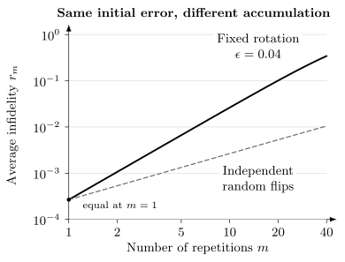
The two devices have the same one-operation infidelity, $r_1=2.67\times10^{-4}$, with $\epsilon=0.04$ radians and $p=\sin^2(0.02)$. The curves show the exact expressions above, not fits. At 40 repetitions they differ by more than a factor of 30. A single fidelity does not specify how errors combine.

Randomized benchmarking averages over randomized gate sequences to reduce sensitivity to fixed state-preparation and measurement errors (Magesan, Gambetta and Emerson, 2011). In the standard gate-independent Markovian model, the fitted survival probability has the form

$$\begin{aligned} P(m)&=A\lambda^m+B,\\ r&=\frac{d-1}{d}(1-\lambda). \end{aligned}$$

Here $d$ is the computational dimension and $r$ refers to the operation sampled by the protocol, often a Clifford rather than one physical pulse. Leakage, drift and temporal correlations require additional treatment. Gate-dependent noise has a more careful interpretation, discussed by Wallman (2018); it does not automatically invalidate an exponential fit. Neither the fit nor a coherence time determines the error of an arbitrary long circuit.

When estimating a cycle error by adding small probabilities, specify the independent stochastic model that permits the addition. Test simultaneous operations when neighboring controls are active. Fault-tolerance thresholds also depend on the circuit, code, decoder and noise model; surface-code terminology explains those distinctions.

Virtual gates and the cost of selective control

A voltage applied near one quantum dot also shifts its neighbors. Linearizing around an operating point gives a response matrix $J_{ij}=\partial O_i/\partial v_j$, where $O_i$ is a measured device parameter. To request a change $\delta\mathbf O$, choose voltages from $J\delta\mathbf v=\delta\mathbf O$. In a square nonsingular case this uses $J^{-1}$; with extra controls, a weighted or constrained solution can respect voltage limits and noise.

These combinations are called virtual gates. Volk and colleagues (2019) used them to compensate first-order shifts of dot electrochemical potentials while extending an array. Compensation of those potentials does not automatically stabilize tunnel barriers; the relevant responses must also be measured.

Conditioning depends on units. First scale voltages by chosen control ranges and observables by desired tolerances, obtaining dimensionless vectors $\mathbf x,\mathbf y$. A simple two-dot example is

$$\mathbf y=C\mathbf x,\qquad C=\begin{pmatrix}1&c\\c&1\end{pmatrix}.$$

Equal changes of the controls have gain $1+c$; opposite changes have gain $1-c$. Thus, for $0\le c<1$,

$$\kappa_2(C)=\frac{1+c}{1-c}.$$

At $c=0.95$, the condition number is 39. A differential target $\mathbf y=(a,-a)$ requires $\mathbf x=(a,-a)/(1-c)$: a modest target can need a large voltage excursion. Small calibration errors then matter strongly, and the excursion may leave the range where the linear model is accurate. A mathematical inverse cannot create a missing physical control direction at $c=1$.

Arrays, defects and cooling

If every component independently works with probability $y$, an array requiring all $N$ components has yield

$$Y=y^N.$$

For $y=0.995$ and $N=1000$, $Y\simeq0.00665$. This is a model of a particular requirement, not a prediction for every architecture. If up to $k$ failed components are usable through redundancy or rerouting, the corresponding independent model is

$$Y_{\le k}=\sum_{j=0}^{k}\binom Nj(1-y)^j y^{N-j}.$$

Connectivity and defect locations can matter more than the count. Correlations also change the answer in either direction: failures shared across an entire wafer produce a different distribution from isolated defects, even at the same marginal component yield. Exercise 4 makes this distinction explicit.

Control wires conduct heat as well as signals. For a uniform wire of area $A$, length $L$, thermal conductivity $\kappa(T)$ and no internal heating, steady one-dimensional Fourier conduction gives

$$\dot Q=\frac{A}{L}\int_{T_c}^{T_h}\kappa(T)\,dT.$$

Thermal anchors break a real line into segments. Resistive losses, attenuators and active electronics add dissipation at their respective stages. Multiplexing reduces some wire counts, but shared bandwidth and added components can change operation times, noise and crosstalk. These physical constraints are developed in Reilly (2015). Increasing qubit density helps only if control, cooling and measurement can support the intended operating cycle.

Exercises

1. Passive reset and throughput

Let $T_1=200\,\mu\mathrm{s}$, $p_e(0)=1$ and $p_{\mathrm{eq}}=0.02$. How long must passive reset wait to reach $p_e=0.03$? If the rest of the sequential cycle takes $20\,\mu\mathrm{s}$, what repetition rate is possible? Can waiting reach 0.01?

Solution

Solving the population equation gives

$$t=T_1\ln\frac{1-0.02}{0.03-0.02} \simeq917\,\mu\mathrm{s}.$$

The total cycle is about $937\,\mu\mathrm{s}$, giving $1.07\,\mathrm{kHz}$. Waiting cannot reach 0.01 because the thermal fixed point is 0.02. The rate assumes sequential operations without overlapping cycles or additional delays.

2. Equal one-operation fidelities

Use the figure’s $\epsilon=0.04$ and matching random-flip probability. Find the average infidelity after 40 operations for both models. Explain why multiplying the one-operation error by 40 misses the coherent result.

Solution

Here $p=\sin^2(0.02)\simeq0.00039995$. Therefore

$$\begin{aligned} r_{40}^{\mathrm{coh}}&=\tfrac23\sin^2(0.8)\simeq0.343,\\ r_{40}^{\mathrm{rand}}&=\tfrac13[1-(1-2p)^{40}]\\ &\simeq0.0105. \end{aligned}$$

The coherent amplitudes retain their relative phase, so their rotation angles add before the final probability is computed. Independent flips instead average over different histories. The ratio is about 32.7.

3. A nearly singular control response

Take $c=0.95$ and the target $\mathbf y=(0.01,-0.01)$. Find $\mathbf x$. If the actual cross-coupling is $0.951$ but the controller uses 0.95, what output results?

Solution

The chosen controls are $\mathbf x=(0.2,-0.2)$. Applying the actual matrix gives $\mathbf y_{\mathrm{actual}}=(0.0098,-0.0098)$. A 0.001 error in $c$ produces a 2% differential-target error. The normalization of both control and output coordinates is part of this calculation; changing units without rescaling the tolerances would change the apparent condition number.

4. Correlated failures

Compare 1000 independent components of yield 0.995 with a fabrication model in which 99.5% of arrays have every component working and 0.5% have none. Do the component yields agree? What are the all-good yields?

Solution

Every component has marginal success probability 0.995 in both models. The independent all-good yield is $0.995^{1000}\simeq0.00665$, whereas the correlated model gives 0.995. Both have five failed components per array on average. That mean hides completely different distributions. Correlations therefore cannot simply be described as always lowering yield; the acceptance condition and joint distribution must be specified.

5. Where a thermal anchor helps

Suppose $\kappa(T)=\kappa_0 T$. Compare a wire of length $L$ from 4 K to 0.02 K with the same wire ideally anchored at its midpoint to 1 K. Assume that the anchor holds 1 K exactly. What is the ratio of the conducted heat arriving at the cold end?

Solution

Without an anchor,

$$\dot Q_0=\frac{A\kappa_0}{2L}(4^2-0.02^2).$$

The cold segment now has length $L/2$ and endpoints 1 K and 0.02 K, so

$$\frac{\dot Q_{\mathrm{cold}}}{\dot Q_0} =\frac{2(1^2-0.02^2)}{4^2-0.02^2} \simeq0.125.$$

The anchor intercepts most of the heat before it reaches the coldest stage. It must itself remove the difference between the hot-segment and cold-segment heat currents; it is not a free heat sink. This idealization omits contact resistance, parasitic heating and temperature dependence beyond the assumed law.

References

• D. Loss and D. P. DiVincenzo, “Quantum Computation with Quantum Dots,” Physical Review A 57, 120–126 (1998), doi:10.1103/PhysRevA.57.120.
• E. Magesan, J. M. Gambetta, and J. Emerson, “Scalable and Robust Randomized Benchmarking of Quantum Processes,” Physical Review Letters 106, 180504 (2011), doi:10.1103/PhysRevLett.106.180504.
• D. J. Reilly, “Engineering the Quantum-Classical Interface of Solid-State Qubits,” npj Quantum Information 1, 15011 (2015), doi:10.1038/npjqi.2015.11.
• C. Volk, A. M. J. Zwerver, U. Mukhopadhyay, P. T. Eendebak, C. J. van Diepen, J. P. Dehollain, T. Hensgens, T. Fujita, C. Reichl, W. Wegscheider, and L. M. K. Vandersypen, “Loading a Quantum-Dot Based ‘Qubyte’ Register,” npj Quantum Information 5, 29 (2019), doi:10.1038/s41534-019-0146-y.
• J. J. Wallman, “Randomized Benchmarking with Gate-Dependent Noise,” Quantum 2, 47 (2018), doi:10.22331/q-2018-01-29-47.