Conductance Quantization

A perfectly transmitted electronic channel contributes $e^2/h$ to two-terminal conductance. When a gate opens transverse modes one at a time, the conductance approaches a staircase. Unresolved spin pairs give the familiar step $G_0=2e^2/h\simeq77.48\,\mu\mathrm S$.

The discrete count concerns transmitting branches, not the number of electrons stored in the device or a bulk conductivity. We derive the elastic, normal-state two-reservoir result, then examine thermal rounding, contacts and what noise can reveal about imperfect channels. Quantum Point Contacts explains how gates form and tune the bottleneck and how it can sense nearby charge.

Required background. Reflection and Transmission Coefficients supplies flux normalization; Chemical Potential and Fermi–Dirac Statistics describe reservoirs; Effective Mass supplies band dispersion and velocity.

Channel flux and the conductance quantum

Let the electron charge be $-e$, with $e>0$, and define $V=(\mu_S-\mu_D)/e$. We take positive $I$ to be conventional charge current from drain to source, opposite to the source-to-drain electron flow. The reservoirs have equilibrium Fermi distributions; the intervening region conserves particle flux and scatters elastically. Strongly interacting or inelastic transport needs additional justification beyond this one-particle description.

For one monotonic right-moving branch in length $L$, momentum spacing $2\pi/L$ gives

$$\frac{dN_+}{L}=\frac{dk}{2\pi}.$$

Using $v=(1/\hbar)dE/dk>0$ gives the density of incoming states per length and energy,

$$\frac1L\frac{dN_+}{dE}=\frac1{hv(E)}.$$

Each state contributes flux proportional to its speed. The two factors cancel:

$$e\,v(E)\frac{dE}{hv(E)}=\frac eh\,dE.$$

A slow branch has more states in the same energy interval. This compensation explains why effective mass does not appear explicitly in the conductance quantum. At an exact band extremum $v=0$, use the limit from propagating energies; do not divide by zero at the isolated threshold itself.

Subtracting the injected source and drain populations yields

$$I=\frac eh\sum_a\int T_a(E)[f_S-f_D]\,dE.$$

The index $a$ includes every spin, valley and other resolved incoming branch. Linearizing the distributions around a common chemical potential gives the Landauer conductance

$$G=\frac{e^2}{h}\sum_a\int T_a(E)w_T(E)\,dE,$$ $$w_T(E)=-\frac{\partial f(E-\mu)}{\partial E}.$$

At zero temperature the normalized kernel becomes $\delta(E-\mu)$, so

$$G=\frac{e^2}{h}\sum_aT_a(\mu).$$

The result is independent of the choice of incoming channel basis. If geometrical modes mix, $T_a$ are eigenvalues of the flux-normalized matrix $t^\dagger t$, where $t$ maps incoming source amplitudes to outgoing drain amplitudes. Flux conservation gives $0\le T_a\le1$. Unitary mixing among perfectly transmitted modes leaves their eigenvalues equal to one; mixing does not itself imply backscattering (Büttiker and colleagues, 1985).

Count branches once

For $N$ perfectly transmitted orbital modes with the same unresolved degeneracy $g_d$,

$$G=g_dN\frac{e^2}{h}.$$

Use either this grouped count or a sum over resolved branches, never both. Degeneracy alone is insufficient if the contacts transmit the branches differently.

Transmitting states opened together	Ideal increment
One resolved branch	$e^2/h$
A spin pair	$2e^2/h$
Two valleys, each with a spin pair	$4e^2/h$
Spin or valley branches split in energy	Separate $e^2/h$ increments

The energy separation must exceed the relevant broadening to resolve separate steps. For a simple Zeeman splitting the scale is $|g^*|\mu_{\mathrm B}B$, but a magnetic field can also change orbital motion and confinement. The numerical value of $G_0$ follows from the exact SI definitions of $e$ and $h$; it does not specify a device’s experimental accuracy (NIST conductance quantum).

A hard-wall example

For a uniform effective-mass guide of width $W$, transverse thresholds are

$$E_n^\perp=\frac{\hbar^2\pi^2n^2}{2m^*W^2}, \qquad n=1,2,\ldots.$$

Count each $n$ with $E_n^\perp<\mu$. Away from exact threshold coincidences, this is $\lfloor k_FW/\pi\rfloor$ when $k_F$ is defined relative to the same band bottom. At $k_FW/\pi=4.28$, four orbital modes fit and ideal spin-degenerate leads give $4G_0$. A depleted constriction requires its local barrier, not an unmodified reservoir density, for this estimate.

For a nonmonotonic subband, count right-moving roots of $E(k)=\mu$, not merely named subbands; Quantum Wires gives a four-root example. Smooth entrances suppress unwanted reflection, but a ballistic impurity-free constriction may still reflect at an abrupt boundary or a barrier top.

Two causes of a rounded riser

An ideal threshold has $T(E)=\Theta(E-E_n)$. Integrating it against the thermal kernel gives

$$\frac{G_n}{g_de^2/h} =\frac1{1+e^{(E_n-\mu)/(k_{\mathrm B}T)}}.$$

Its 10–90 percent width in energy is $2k_{\mathrm B}T\ln9\simeq4.394k_{\mathrm B}T$. Temperature averages a fixed transmission curve; it does not automatically change that curve itself. Heating may additionally change the physical device.

A smooth saddle already rounds transmission at zero temperature. For its longitudinal inverted oscillator, write $s=\hbar\omega_x/(2\pi)$:

$$T_n(E)=\frac1{1+e^{-(E-E_n)/s}}.$$

The corresponding 10–90 percent width is $2s\ln9$. The transverse spacing is $\hbar\omega_y$ in the separable harmonic model. This result comes from matching the scattering solutions of the inverted oscillator (Büttiker, 1990); the local potential and mode assumptions are developed in Quantum Point Contacts.

At finite temperature, convolve the saddle transmission with $w_T$. Adding the two 10–90 widths, or combining them in quadrature, is not an exact rule. Resolving plateaus requires the resulting risers to be narrow compared with the threshold spacing. A gate-voltage width becomes an energy width only after determining a local lever arm, $dE_n=-\alpha e\,dV_g$.

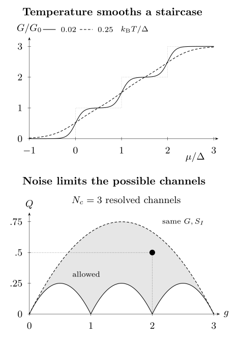
Top: three equally spaced spin-degenerate thresholds, separated by $\Delta$, with saddle scale $s=0.08\Delta$. The curves are thermal convolutions at $k_{\mathrm B}T/\Delta=0.02$ and $0.25$; the dotted curve is the ideal sharp staircase. Bottom: allowed zero-temperature noise quantity $Q=\sum_aT_a(1-T_a)$ for three resolved channels at fixed $g=\sum_aT_a$. Different transmission sets can share both $g$ and $Q$; the marked point is the counterexample below. These calculated models illustrate rounding and inference limits, not measured data.

Finite bias can move the transmission curve

At zero temperature and positive $V$, the occupied transport window gives

$$I=\frac eh\sum_a\int_{\mu_D}^{\mu_S}T_a(E,V)\,dE.$$

Take $d\mu_S/dV=\eta e$ and $d\mu_D/dV=-(1-\eta)e$. Differentiating includes both moving endpoints and any bias response of the scatterer:

$$\frac{dI}{dV}=\frac{e^2}{h}\sum_a \big[\eta T_a(\mu_S,V) +(1-\eta)T_a(\mu_D,V)\big] +\frac eh\sum_a\int_{\mu_D}^{\mu_S} \partial_VT_a(E,V)\,dE.$$

For a rigid scatterer and symmetric bias, the last term vanishes and the endpoint weights are $1/2$. A single resolved threshold between the two potentials then contributes $e^2/(2h)$ to differential conductance. It need not contribute that value to $I/V$.

If instead a threshold shifts by $\beta eV$, with its shape otherwise fixed, then $\partial_VT=-\beta e\partial_ET$. The endpoint weights become $\eta-\beta$ and $1-\eta+\beta$. This is why a half-step is conditional, even with geometrically symmetric contacts. Heating, resonances and interacting nonlinear response require further modeling. Quantum Point Contacts connects these parameters to spectroscopy ridges.

Contacts explain a finite resistance without reflection

A single resolved channel has two-terminal resistance

$$R_2=\frac{h}{e^2T}.$$

It remains $h/e^2$ at $T=1$. The reservoirs supply incoming populations at different electrochemical potentials; a reflectionless interior does not remove this injection resistance. In the elastic model the outgoing distributions relax in reservoirs, where heat is released. The location and division of heating depend on the energy distribution; one should not infer a uniform local resistivity from $R_2$.

A specified four-probe limit

There is no universal four-terminal resistance without a probe model (Büttiker, 1986). For illustration, attach weak probes on each side that sample right- and left-moving populations equally, with standing-wave interference averaged out. Take linear response and energy-independent $T$, and write $R=1-T$. Zero probe current sets

$$\mu_L^{p}=\frac{(1+R)\mu_S+T\mu_D}{2},$$ $$\mu_R^{p}=\frac{T\mu_S+(1+R)\mu_D}{2}.$$

Their difference is $R(\mu_S-\mu_D)$, so this particular voltage measurement yields

$$R_4=\frac{h}{e^2}\frac{1-T}{T}.$$

It vanishes at perfect transmission. A coherent local probe with unequal coupling to the directions, or an invasive equilibrating contact, can give a different result. Multichannel probe readings likewise require their actual coupling; do not add single-channel $R_4$ values as resistors in series.

An ordinary external series resistance instead gives $G_{\rm meas}^{-1}=R_s+G_{\rm device}^{-1}$. Determine $R_s$ independently. Adjusting it solely to manufacture integer plateaus cannot test quantization.

Noise constrains imperfect channels

At zero temperature, a resolved channel supplies approximately $M=e|V|\tau/h$ occupied incident states during a long counting time $\tau$. Independent elastic partitioning gives mean transmitted count $MT_a$ and variance $MT_a(1-T_a)$. Therefore the one-sided low-frequency current spectrum is

$$S_I^{(1)}=\frac{2e^2}{h}\,e|V|\,Q,$$ $$g=\sum_aT_a,\qquad Q=\sum_aT_a(1-T_a).$$

Here $G=(e^2/h)g$ and the Fano factor is $F=Q/g$ for nonzero current. The factor of two matches the one-sided spectrum per ordinary frequency; a Poisson stream has $S_I^{(1)}=2e|I|$.

For energy-independent channels at common temperature, define

$$\mathcal E(V,T)=e|V|\coth\frac{e|V|}{2k_{\mathrm B}T}.$$

Then the thermal-to-shot-noise crossover is

$$S_I^{(1)}=4k_{\mathrm B}TG +\frac{2e^2}{h}Q[\mathcal E-2k_{\mathrm B}T].$$

The continuous $V\to0$ limit has $\mathcal E\to2k_{\mathrm B}T$, giving Johnson noise $4k_{\mathrm B}TG$. A perfect channel eliminates the partition contribution, not thermal noise. Strong energy dependence requires the full energy integral rather than this crossover formula (Blanter and Büttiker, 2000).

Two moments do not generally fix every channel

Conductance gives $\sum T_a$, while noise gives $\sum T_a^2=g-Q$. For three channels the sets

$$(T_1,T_2,T_3)=(1,1/2,1/2)$$

and

$$(T_1,T_2,T_3)=(5/6,5/6,1/3)$$

both give $g=2$, $Q=1/2$ and $F=1/4$. One contains a perfect channel and the other does not. Thus even an integer conductance plus measured noise need not identify the full transmission spectrum.

For a known number $N_c$ of resolved channels, the allowed interval is

$$r(1-r)\le Q\le g\left(1-\frac{g}{N_c}\right),$$

where $r=g-\lfloor g\rfloor$ and $0\le g\le N_c$. The upper bound follows from Cauchy–Schwarz and is reached by equal transmissions. The lower bound is reached by as many unit transmissions as possible, one fractional remainder, and zeros. In particular, zero partition noise forces every transmission to be zero or one under these assumptions. Small positive noise constrains, but does not uniquely reconstruct, their departures from those endpoints.

Compare the staircase with experiments

Van Wees and colleagues and Wharam and colleagues independently observed steps near $2e^2/h$ in gate-defined GaAs/AlGaAs constrictions in 1988. The mode picture connects their step scale to spin pairs and transverse confinement. Temperature sweeps, finite-bias spectroscopy, magnetic splitting and noise test different parts of that interpretation.

Atomic contacts require a different geometrical picture: their transmission channels reflect chemical valence orbitals, and atomic rearrangements can also make steps. Scheer and colleagues (1998) used superconducting subgap characteristics to extract individual normal-state transmissions. A conductance histogram peaked near an integer alone does not perform that reconstruction.

The 0.7 shoulder and other departures

A shoulder near $0.7G_0$ below the first semiconductor plateau is sensitive to interactions, spin and device conditions. It is not an additional threshold in the elementary noninteracting model. Micolich (2011) reviews the temperature, bias and magnetic-field comparisons that distinguish proposed explanations. A particular shoulder does not by itself establish static spin polarization or fractional quasiparticles.

Chiral Hall edges and superconducting contacts also use channel language, but with different transport mechanisms. Integer Quantum Hall Effect includes topology, localization and terminal equilibration; Proximity and Andreev Physics includes electron–hole conversion. Numerical equality of a conductance value does not identify its mechanism.

Exercises

1. Turn a thermal width into a gate width. For an otherwise ideal threshold at $100\,\mathrm{mK}$, find the 10–90 percent energy width. Use $dE_n=-0.050e\,dV_g$ to convert it to gate voltage.

Solution

The normalized logistic riser reaches $p$ when $\mu-E_n=k_{\mathrm B}T\ln[p/(1-p)]$. Subtracting the values at $0.1$ and $0.9$ gives $2k_{\mathrm B}T\ln9=37.9\,\mu\mathrm{eV}$. The voltage width is $0.757\,\mathrm{mV}$. This is the purely thermal result; an intrinsic saddle width must be convolved with the thermal kernel.

2. Moving-barrier half-step. At zero temperature, a resolved ideal threshold lies strictly inside the bias window. Take $\eta=1/2$ and a threshold shift $\beta eV$ with $\beta=0.20$. Find its differential conductance.

Solution

For positive $V$, the transmitted interval has length $\mu_S-E_n(V)$. Its derivative is $(\eta-\beta)e$, giving $dI/dV=0.30e^2/h$. Dropping the barrier derivative would incorrectly give $0.50e^2/h$. The result applies only while the threshold stays inside the window and the rigid-shift model holds.

3. Mixing without reflection. Two incoming channels are transmitted through an arbitrary $2\times2$ unitary matrix $U$. Find the conductance and partition noise. What changes if the transmission block is $t=U\operatorname{diag}(1,\sqrt{0.4})$?

Solution

For $t=U$, $t^\dagger t=I$, giving $G=2e^2/h$ and $Q=0$. The outgoing modes may be completely mixed. In the second case the eigenvalues are $1$ and $0.4$, so $G=1.4e^2/h$, $Q=0.24$ and $F=0.24/1.4\simeq0.171$. The unitary rotation changes neither result.

4. Compare voltage measurements. For one resolved channel with $T=0.8$, compare $R_2$ with the equal-direction weak-probe $R_4$ derived above. Why is their difference not ordinary impurity resistance?

Solution

The two values are $1.25h/e^2$ and $0.25h/e^2$. Their difference $h/e^2$ is the injection contribution for this setup. It remains even as reflection vanishes. The conclusion depends on the specified probe coupling; a general coherent four-terminal experiment requires its scattering matrix.

5. What would distinguish the noise counterexample? Verify that the two three-channel sets in the text share $g$ and $Q$. Compare the third transmitted-count cumulant per incident-state opportunity,

$$C_3=\sum_aT_a(1-T_a)(1-2T_a).$$

Solution

Both have sum $2$ and squared sum $3/2$, hence $Q=1/2$. For $(1,1/2,1/2)$ every third-cumulant term vanishes. For $(5/6,5/6,1/3)$,

$$C_3=-\frac5{27}+\frac2{27}=-\frac19.$$

The third cumulant distinguishes these ideal examples. In a measurement, finite temperature, energy dependence and environmental feedback must be included before interpreting higher cumulants as transmission moments.

References

• Ya. M. Blanter and M. Büttiker, “Shot Noise in Mesoscopic Conductors,” Physics Reports 336, 1–166 (2000), doi:10.1016/S0370-1573(99)00123-4, arXiv:cond-mat/9910158.
• M. Büttiker, “Four-Terminal Phase-Coherent Conductance,” Physical Review Letters 57, 1761–1764 (1986), doi:10.1103/PhysRevLett.57.1761.
• M. Büttiker, “Quantized Transmission of a Saddle-Point Constriction,” Physical Review B 41, 7906–7909 (1990), doi:10.1103/PhysRevB.41.7906.
• M. Büttiker, Y. Imry, R. Landauer and S. Pinhas, “Generalized Many-Channel Conductance Formula with Application to Small Rings,” Physical Review B 31, 6207–6215 (1985), doi:10.1103/PhysRevB.31.6207.
• A. P. Micolich, “What Lurks Below the Last Plateau: Experimental Studies of the 0.7 × 2e²/h Conductance Anomaly in One-Dimensional Systems,” Journal of Physics: Condensed Matter 23, 443201 (2011), doi:10.1088/0953-8984/23/44/443201, arXiv:1110.3474.
• National Institute of Standards and Technology, “Conductance Quantum,” CODATA 2022 Values, constant entry (accessed 15 October 2026).
• E. Scheer, N. Agraït, J. C. Cuevas, A. Levy Yeyati, B. Ludoph, A. Martín-Rodero, G. Rubio Bollinger, J. M. van Ruitenbeek and C. Urbina, “The Signature of Chemical Valence in the Electrical Conduction through a Single-Atom Contact,” Nature 394, 154–157 (1998), doi:10.1038/28112.
• B. J. van Wees, H. van Houten, C. W. J. Beenakker, J. G. Williamson, L. P. Kouwenhoven, D. van der Marel and C. T. Foxon, “Quantized Conductance of Point Contacts in a Two-Dimensional Electron Gas,” Physical Review Letters 60, 848–850 (1988), doi:10.1103/PhysRevLett.60.848.
• D. A. Wharam, T. J. Thornton, R. Newbury, M. Pepper, H. Ahmed, J. E. F. Frost, D. G. Hasko, D. C. Peacock, D. A. Ritchie and G. A. C. Jones, “One-Dimensional Transport and the Quantisation of the Ballistic Resistance,” Journal of Physics C: Solid State Physics 21, L209–L214 (1988), doi:10.1088/0022-3719/21/8/002.