Universal Conductance Fluctuations

Universal conductance fluctuations are reproducible, sample-specific changes in the conductance of a coherent disordered conductor as field, energy, or disorder configuration varies. In a fully coherent diffusive metal, their root-mean-square scale is of order $e^2/h$. “Universal” describes the variance within a specified geometry and symmetry class, not the detailed peaks of a trace or an exact amplitude of $e^2/h$.

The word fluctuations need not mean temporal noise. With frozen disorder, repeated field sweeps reproduce the same irregular magnetofingerprint. A moving defect can change that fingerprint, but the defect’s motion and the coherent conductor’s sensitivity to it are distinct questions.

Required background. Mesoscopic scales distinguish device size, mean free path and thermal length; quantum coherence separates phase loss from averaging; conductance quantization provides the transmission-channel formula.

A fixed sample has a fixed interference pattern

For a normal conductor in linear response, count every spin and valley channel in $t$ and write

$$G=\frac{e^2}{h}g, \qquad g=\operatorname{Tr}(t^\dagger t).$$

Each transmission amplitude sums many elastic scattering paths. Squaring it produces path-pair interference terms. Their phases remain fixed when the disorder is fixed: elastic scattering randomizes momentum without necessarily erasing phase. A field change $\Delta B$ changes a pair’s magnetic phase by $-2\pi\Delta B\mathcal A/\Phi_0$, where $\mathcal A$ is its oriented enclosed area and $\Phi_0=h/e$. An energy change instead shifts its dynamical phase by approximately $\Delta E\,\Delta t/\hbar$, where $\Delta t$ is the difference of traversal times.

Different pairs enclose different areas and have different delays. Their sum is irregular rather than a single periodic oscillation. Normal-metal rings and wires show such reproducible structure (Umbach and colleagues, 1984). Sensitivity to moving scatterers can also produce time-dependent noise when the disorder evolves (Feng, Lee, and Stone, 1986).

Define the fluctuation relative to the disorder-ensemble mean:

$$\delta G(X)=G(X)-\langle G(X)\rangle_{\rm dis}.$$

Then $\langle\delta G\rangle_{\rm dis}=0$, while its variance is nonzero. In one device, subtracting a smooth fitted background approximates this separation. It is an additional analysis step whose effect must be checked.

Why the variance has a quantum scale

The metallic diffusive regime requires $\ell\ll L\ll\xi$, $k_F\ell\gg1$ and $\langle g\rangle\gg1$. Here $\ell$ is the elastic mean free path and $\xi$ the localization length. To avoid substantial phase loss and energy averaging, also require $L\lesssim L_\phi$ and $k_BT\ll E_{\rm Th}$, with $E_{\rm Th}=\hbar D/L^2$.

The many transmission probabilities are correlated: treating them as independent classical contributions gives the wrong variance. Long-lived diffusion modes retain correlations between interfering amplitudes (Lee and Stone, 1985; Lee, Stone, and Fukuyama, 1987).

For one spinless block in a long, narrow diffusive wire with ideal absorbing leads, those modes have $q_n=n\pi/L$, $n\geq1$. The zero-temperature mode sum is

$$\begin{aligned} \operatorname{var}g &=\frac{12}{\beta L^4}\sum_{n=1}^{\infty}\frac{1}{q_n^4}\\ &=\frac{12}{\beta\pi^4}\sum_{n=1}^{\infty}\frac{1}{n^4}\\ &=\frac{2}{15\beta}. \end{aligned}$$

The prefactor comes from the conductance correlation calculation; a mode count alone does not derive it. The sum makes the cancellation of $L$ explicit, and $D$ has likewise canceled between the diffusion poles and current factors. Boundary conditions exclude the zero mode because electrons escape through the leads. This is the quasi-one-dimensional benchmark, not a formula for any shape (Beenakker, 1997; Montambaux, 2016).

For this spinless block, $\beta=1$ with time-reversal symmetry and $\beta=2$ when orbital magnetic field breaks it. The rms values are respectively $0.365\,e^2/h$ and $0.258\,e^2/h$. Breaking the symmetry halves the variance, reducing the rms by $1/\sqrt2$. A ballistic chaotic cavity has a different coefficient; localized transport is outside this metallic approximation.

Degenerate channels can carry the same fluctuation

If two spin blocks are identical, $g=2g_0$ and their variances add coherently: $\operatorname{var}g=4\operatorname{var}g_0$. If they are statistically independent, the factor is two instead. More generally, for equal single-block variance $v$ and correlation coefficient $\rho$,

$$\operatorname{var}(g_1+g_2)=2v(1+\rho).$$

Resolving two channel labels does not make them independent. Zeeman splitting can decorrelate spin fingerprints when it exceeds their energy correlation scale; spin–orbit and intervalley scattering change the relevant diffusion modes. Apply the symmetry class, degeneracy and conductance unit together. In particular, do not insert a symplectic index into the spinless formula while leaving Kramers counting unspecified.

Field correlations and reciprocity

The full covariance is a function of two fields,

$$C(B,B')=\langle\delta G(B)\delta G(B')\rangle_{\rm dis}.$$

In the diffusive description, diffuson terms depend on the field difference $B-B'$, whereas Cooperon terms depend on the sum $B+B'$. The latter pair amplitudes related by time reversal. At equal fields the diffuson remains, while a sufficiently large mean field suppresses the Cooperon. This gives the simplest factor-of-two crossover. It also means a window spanning that crossover is not statistically stationary: its variance changes with position.

For a two-terminal linear measurement, reciprocity gives $G(B)=G(-B)$ when all other time-reversal-odd controls are absent or reversed. Consequently the negative-field half duplicates the positive-field half. Multiterminal reciprocity instead exchanges current and voltage leads; it need not make one fixed lead arrangement even.

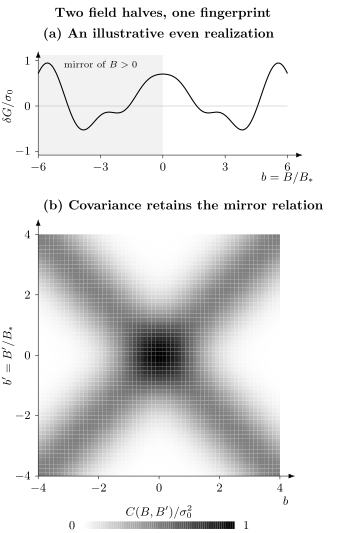
A statistical illustration of reciprocity, not a microscopic prediction for a particular wire. The covariance is $C/\sigma_0^2=[k(b-b')+k(b+b')]/2$, with $k(x)=e^{-x^2/2}$ and $b=B/B_*$. A Gaussian random cosine sum generates the trace. The covariance map has a ridge at $B'=B$ and an equally strong mirror ridge at $B'=-B$. At zero field its variance is $\sigma_0^2$, while far from zero it tends to $\sigma_0^2/2$. Actual diffusion geometry determines a different detailed line shape.

Within a sufficiently stationary one-sided window, use the lag covariance $C_B(\Delta B)$. A common width convention is

$$\begin{aligned} C_B(B_c)&=\tfrac12 C_B(0),\\ \operatorname{rms}\delta G&=\sqrt{C_B(0)}. \end{aligned}$$

Keep the dimensional covariance before normalizing it. A half-height width, a first zero and an integral correlation scale are different quantities.

The scale comes from flux through typical coherent loop areas:

$$B_c\sim\alpha\frac{\Phi_0}{A_\phi}.$$

For a narrow wire in perpendicular field, $A_\phi\sim wL_{\rm eff}$; for a two-dimensional patch, $A_\phi\sim L_{\rm eff}^2$. The length $L_{\rm eff}$ is limited by dephasing and the device or escape geometry. When $L_\phi$ exceeds the device, the width saturates at a size-dependent scale rather than continuing to measure $L_\phi$. The coefficient $\alpha$ depends on geometry, boundary conditions, temperature and the width convention; it is not universally one.

Finite coherence and temperature

Combining many coherent regions

Consider a long narrow wire consisting approximately of $M=L/L_\phi$ independent coherent segments, each with mean conductance $G_s$ and small fluctuation $\delta G_i$. Expanding their series resistance gives

$$\delta G_{\rm wire}\simeq\frac{1}{M^2}\sum_{i=1}^M\delta G_i.$$

Independent segment variances then give an rms suppression $M^{-3/2}$. Thus, when thermal averaging is weak,

$$\operatorname{rms}\delta G\sim C_1\frac{e^2}{h} \left(\frac{L_\phi}{L}\right)^{3/2}.$$

This argument explains the exponent, not a precise prefactor: real dephasing is not an array of artificial reservoirs. For a roughly hypercubic $d$-dimensional conductor, series and parallel composition instead gives the exponent $(4-d)/2$. Actual aspect ratios matter.

Average the covariance over energy

Let $w_T(E)=-\partial_E f(E)$, normalized to integrate to one. Thermal conductance is the weighted average of the coherent fingerprint, so its variance is

$$\begin{aligned} \operatorname{var}G_T&=\int dE\,w_T(E)\mathcal K_T(E),\\ \mathcal K_T(E)&=\int dE'\,w_T(E')C_E(E-E'). \end{aligned}$$

The inner integral $\mathcal K_T(E)$ averages the correlation with energy $E$ over the second energy. This expression assumes the underlying energy covariance is approximately stationary across the thermal window and holds its dephasing parameters fixed. It is a double average of a covariance, not an average of the rms amplitude. If $C_E$ is short-ranged compared with $k_BT$, then

$$\operatorname{var}G_T\simeq \frac{1}{6k_BT}\int d\varepsilon\,C_E(\varepsilon),$$

using $\int w_T^2dE=1/(6k_BT)$. Thus a variance of typical width $E_c$ is reduced by a factor of order $E_c/(k_BT)$, with a line-shape-dependent coefficient. The rms reduction is its square root. Temperature can separately shorten $\tau_\phi$; the two effects should not be conflated.

In a long quasi-one-dimensional wire, $E_c\sim\hbar D/L_\phi^2$ and $L_T=\sqrt{\hbar D/(k_BT)}$. Combining the spatial and thermal factors gives

$$\operatorname{rms}\delta G\sim C_T\frac{e^2}{h} \frac{L_T L_\phi^{1/2}}{L^{3/2}},$$

when $\ell\ll L_T\ll L_\phi\ll L$, with both transverse dimensions sufficiently small. Thermal averaging can also change the measured field-correlation shape; an unchanged or changing $B_c$ alone is not a complete separation of thermal averaging from dephasing.

For an energy or gate sweep, first establish $\Delta E=\alpha_g e\Delta V_g$ and a roughly stationary device. A gate can also change density, contact transmission and the disorder potential. Finite bias additionally changes reservoir occupations, electrostatics and possibly electron temperature; replacing $k_BT$ by $e|V|$ is not a general theory of nonlinear fluctuations.

Estimating a variance from one trace

Replacing a disorder ensemble by a field or gate sweep is an ergodic assumption. It is most useful when the trace spans many correlation scales without changing its transport regime. Repeating a sweep tests reproducibility; it does not create a new independent disorder sample.

A finite window also biases mean subtraction. For a stationary zero-mean fluctuation $x(B)$ on $0<B<W$, let $\bar x=W^{-1}\int_0^W x(B)dB$ and estimate

$$\widehat V=\frac1W\int_0^W[x(B)-\bar x]^2dB.$$

Taking the ensemble average yields

$$\begin{aligned} \langle\widehat V\rangle&=C_B(0)-\langle\bar x^2\rangle,\\ \langle\bar x^2\rangle&=\frac{2}{W^2} \int_0^W(W-u)C_B(u)\,du. \end{aligned}$$

Even subtracting a constant removes some fluctuation power. A flexible polynomial or a smoothing window comparable to $B_c$ removes more. Sampling the same window more finely does not undo this bias or supply more independent features. Compare results from defensible backgrounds and subwindows; uncertainty depends on correlation tails as well as a nominal $W/B_c$ count.

A fixed external series resistance also suppresses the fluctuation. If $G_m=G_s/(1+R_sG_s)$, then for small sample fluctuations

$$\delta G_m=\frac{\delta G_s}{(1+R_s\overline G_s)^2}.$$

Correct the measurement convention before comparing with an ideal-lead variance. A four-terminal resistance is not generally the inverse of a two-terminal conductance.

Structure in a trace	Distinguishing comparison
Universal conductance fluctuations	Reproducible, aperiodic field or energy covariance
Aharonov–Bohm oscillations	Harmonics periodic in enclosed flux
Weak localization	Ensemble-averaged low-field correction
Landau-level oscillations	Typically periodic in $1/B$
Temporal noise	Changes at fixed controls; analyze time correlations

Several effects can coexist. Agreement of the regime, reproducibility, correlation scales and temperature dependence is more informative than labeling every irregular feature UCF. Nor does an order-$e^2/h$ signal alone identify topological boundary transport.

Exercises

1. Count correlated spin blocks

A spinless orthogonal wire has variance $v=2/15$ in units of $(e^2/h)^2$. Find the total rms for two identical blocks, two independent blocks, and two blocks with $\rho=1/2$.

Solution

The variances are $4v$, $2v$ and $3v$, respectively. The rms values are $0.730$, $0.516$ and $0.632$ times $e^2/h$. All three cases have two blocks; their statistical correlation changes the answer. An orbital symmetry crossover and a spin-decorrelation crossover need not occur at the same field.

2. Derive the wire-length suppression

Expand $G_{\rm wire}=[\sum_i(G_s+\delta G_i)^{-1}]^{-1}$ to first order. For $M=4$ independent segments of rms $s$, find the wire rms. What if all segment fluctuations were identical?

Solution

Expanding the resistance and then inverting gives

$$G_{\rm wire}\simeq\frac{G_s}{M} +\frac{1}{M^2}\sum_i\delta G_i.$$

Independent fluctuations have sum variance $Ms^2$, giving rms $s/M^{3/2}=s/8$. Identical fluctuations instead have sum variance $M^2s^2$, giving $s/M=s/4$. Independence is the physical assumption behind the $3/2$ exponent.

3. Thermal averaging of an energy fingerprint

For the illustrative energy covariance $C_E(\varepsilon)=\sigma^2e^{-\varepsilon^2/(2E_c^2)}$, find the leading variance and rms for $k_BT\gg E_c$. Does this determine a dephasing rate?

Solution

The Gaussian area is $\sqrt{2\pi}\sigma^2E_c$, so

$$\begin{aligned} \operatorname{var}G_T&\simeq \frac{\sqrt{2\pi}}6\sigma^2\frac{E_c}{k_BT},\\ \operatorname{rms}\delta G_T&\simeq 0.646\,\sigma\sqrt{\frac{E_c}{k_BT}}. \end{aligned}$$

This is a high-temperature asymptote for the stated covariance, not a UCF line shape valid in every geometry. The underlying coherence was held fixed; no dephasing rate follows from this calculation alone.

4. Bias from a finite window

Let a stationary field covariance be $C_B(u)=\sigma^2e^{-u^2/(2b^2)}$. Show that subtracting the window mean over $W=10b$ gives approximately $\langle\widehat V\rangle=0.769\sigma^2$. Would doubling the number of sample points fix this?

Solution

With $a=W/b$, the fractional removed variance is

$$\frac{\langle\bar x^2\rangle}{\sigma^2} =\frac{\sqrt{2\pi}}{a}\operatorname{erf}(a/\sqrt2) -\frac{2}{a^2}(1-e^{-a^2/2}).$$

At $a=10$ this is $0.23066$. Therefore the mean estimated variance is $0.76934\sigma^2$. Taking a denser set of measurements in the same window approaches this biased continuum result more accurately. It does not enlarge the statistical sample. The formula assumes stationarity; a window across the field-symmetry crossover needs the full two-field covariance instead.

5. Check a coherence estimate before trusting it

A wire has width $w=100\,\mathrm{nm}$ and length $L=1.0\,\mu\mathrm m$. A fit gives $B_c=0.020\,\mathrm T$. The estimate $L_\phi=\Phi_0/(wB_c)$ gives what length, and why is it questionable? Separately, if $R_s\overline G_s=0.5$, how much does series resistance reduce the measured rms?

Solution

The nominal length is $2.07\,\mu\mathrm m$, exceeding the device length. The assumed dephasing-limited area $wL_\phi$ is then inappropriate; device escape and the geometry coefficient must be included. The measured width may only constrain a coherence length longer than the sample.

The series-resistance rms factor is $(1+0.5)^{-2}=4/9$. The variance is reduced by $(4/9)^2=16/81$. Confusing rms with variance would give the wrong correction.

References

• C. W. J. Beenakker, “Random-Matrix Theory of Quantum Transport,” Reviews of Modern Physics 69, 731–808 (1997), doi:10.1103/RevModPhys.69.731, author manuscript.
• S. Feng, P. A. Lee, and A. D. Stone, “Sensitivity of the Conductance of a Disordered Metal to the Motion of a Single Atom: Implications for $1/f$ Noise,” Physical Review Letters 56, 1960–1963 (1986), doi:10.1103/PhysRevLett.56.1960.
• P. A. Lee and A. D. Stone, “Universal Conductance Fluctuations in Metals,” Physical Review Letters 55, 1622–1625 (1985), doi:10.1103/PhysRevLett.55.1622.
• P. A. Lee, A. D. Stone, and H. Fukuyama, “Universal Conductance Fluctuations in Metals: Effects of Finite Temperature, Interactions, and Magnetic Field,” Physical Review B 35, 1039–1070 (1987), doi:10.1103/PhysRevB.35.1039.
• G. Montambaux, “Disorder and Mesoscopic Physics,” Lecture 4, Cargèse School (2016), author lecture slides.
• C. P. Umbach, S. Washburn, R. B. Laibowitz, and R. A. Webb, “Magnetoresistance of Small, Quasi-One-Dimensional, Normal-Metal Rings and Lines,” Physical Review B 30, 4048–4051 (1984), doi:10.1103/PhysRevB.30.4048.