Two-Dimensional Electron Gases

A two-dimensional electron gas (2DEG) is a populated electronic layer whose low-energy motion is extended in two directions and restricted to confinement subbands in the third. Its density fixes the occupied momentum states, while its thickness, interactions and disorder determine how those states respond. “Gas” does not imply that interactions are negligible.

Semiconductor interfaces provide a controlled starting point. We first use a parabolic conduction band, then examine why multiband transport, spin–orbit coupling and oxide interfaces require additional care. Quantum Wells develops the underlying confinement; Graphene and Dirac Materials treats linear rather than parabolic dispersion.

Required background. Quantum Wells supplies subbands, Fermi Momentum and Fermi Energy supplies state counting, Boltzmann Transport supplies scattering rates, and Hall Effect supplies signed transverse response.

Confined carriers and occupied momentum states

Let $\varepsilon_1<\varepsilon_2$ be the first two confinement thresholds and $\mu$ the chemical potential. At zero temperature only the lowest subband is occupied when $\varepsilon_1<\mu<\varepsilon_2$. At finite temperature, a safely negligible second-subband population requires

$$\varepsilon_2-\mu\gg k_{\mathrm B}T,$$

along with sufficiently weak spectral broadening. Comparing temperature only with $\varepsilon_2-\varepsilon_1$ misses carriers near the second threshold. A layer with several occupied subbands can still be quasi-two-dimensional; it simply needs several populations in the model. The occupation formula in Quantum Wells quantifies the crossover.

Confinement spectroscopy, a bounded carrier depth profile and perpendicular-field scaling provide complementary tests of dimensionality. Sheet conductance or field-angle dependence alone can be imitated by an anisotropic three-dimensional conductor.

For one circular parabolic subband, with $g$ identical unresolved spin or valley branches, the zero-temperature relations are

$$n_s=\frac{gk_F^2}{4\pi}, \qquad \lambda_F=\frac{2\pi}{k_F},$$ $$E_F-\varepsilon_1=\frac{\hbar^2 k_F^2}{2m^*},$$ $$v_F=\frac{\hbar k_F}{m^*}.$$

More generally, an occupied momentum region of area $A_F$ contains

$$n_s=\frac{gA_F}{4\pi^2}.$$

This area count does not require a circle. Measuring one directional radius and assuming circularity can give the wrong area; measuring the correct occupied area and multiplicity gives the correct band-state count. Sum distinct occupied regions separately. An annulus requires an outer area minus an inner area, as the spin–orbit example below illustrates.

For $n_s=3.0\times10^{11}\,\mathrm{cm}^{-2}$, $g=2$ and $m^*=0.067m_e$, these formulas give $\lambda_F=45.8\,\mathrm{nm}$ and $E_F-\varepsilon_1=10.7\,\mathrm{meV}$. The energy is measured from the subband bottom, not from an arbitrary laboratory zero.

Coulomb and screening scales

With absolute dielectric permittivity $\epsilon$ and $e>0$, define

$$a_B^*=\frac{4\pi\epsilon\hbar^2}{m^*e^2},$$ $$r_s=\frac{1}{a_B^*\sqrt{\pi n_s}}.$$

The mean-spacing Coulomb energy $e^2\sqrt{\pi n_s}/(4\pi\epsilon)$ divided by $E_F-\varepsilon_1$ is $(g/2)r_s$. Thus $r_s$ itself is this ratio for $g=2$. It indicates the importance of correlations, not a particular phase.

For a zero-temperature, zero-thickness parabolic gas, the static random-phase approximation gives $q_{\rm TF}=g/a_B^*$ with $V(q)=e^2/(2\epsilon q)$; the underlying polarizability is constant for $q<2k_F$ (Stern, 1967). Density still changes $q_{\rm TF}/k_F$, and finite thickness, multiple bands and correlations modify the response. See Plasmons for collective charge motion.

Interface fields and finite thickness

An impenetrable interface at $z=0$ and a potential $V(z)=e\mathcal E z$ for $z>0$ give a useful triangular-well model. Its natural length and bound energies are

$$\ell_z=\left(\frac{\hbar^2}{2m_z^*e\mathcal E}\right)^{1/3},$$ $$\varepsilon_n=a_n e\mathcal E\ell_z,$$

where $\operatorname{Ai}(-a_n)=0$ and $a_1\simeq2.338$. Increasing the confining field narrows the wavefunction and raises its energy. Actual interface fields depend on the electron population, donors and gates, so quantitative calculations solve the confinement and electrostatics together (Ando, Fowler and Stern, 1982).

The normalized Fang–Howard trial envelope is

$$\chi(z)=\sqrt{\frac{b^3}{2}}\,z e^{-bz/2}, \qquad z\ge0.$$

Its mean penetration is $\langle z\rangle=3/b$, while its root-mean-square width about that mean is $w=\sqrt3/b$. These are different measures of thickness. The parameter $b$ follows from a specified variational electrostatic model (Fang and Howard, 1966).

Projecting a homogeneous-dielectric Coulomb interaction into this envelope gives $V_{\rm eff}(q)=V(q)\mathcal F(q)$, where, with $p(z)=|\chi(z)|^2$,

$$\mathcal F(q)=\int dz\,dz'\,p(z)p(z')e^{-q|z-z'|}.$$

For this profile, write $u=q/b$. Direct integration gives

$$\mathcal F(q)=\frac{1+9u/8+3u^2/8}{(1+u)^3}.$$

Long wavelengths see the total sheet charge: $\mathcal F(0)=1$. Short wavelengths resolve its thickness and the interaction weakens. Dielectric interfaces require the appropriate electrostatic kernel instead of simply inserting this expression. Finite width also permits an orbital response to a parallel magnetic field; strictly two-dimensional kinematics do not make that response vanish identically.

Modulation doping separates electrons from ionized donors, reducing their scattering. Remote charges still produce smooth disorder, and changing the donor setback can change confinement and density too. Undoped gated layers avoid that donor population but retain possible background impurities, interface roughness and fluctuating gate or surface charge.

Mobility and quantum lifetime measure different scattering

For one isotropic parabolic band in the Drude regime,

$$\sigma_\square=n_s e\mu_{\rm mob},$$ $$\mu_{\rm mob}=\frac{e\tau_{\rm tr}}{m^*},$$

and $\ell_{\rm tr}=v_F\tau_{\rm tr}$. We distinguish mobility $\mu_{\rm mob}$ from chemical potential $\mu$. The example above, with mobility $10^6\,\mathrm{cm^2/(V\,s)}$, has $\tau_{\rm tr}=38.1\,\mathrm{ps}$ and $\ell_{\rm tr}=9.04\,\mu\mathrm m$.

For independent elastic scattering on a circular contour, normalize the differential rate $W(\theta)$ so that

$$\frac1{\tau_q}=\int_0^{2\pi}W(\theta)\,d\theta,$$ $$\frac1{\tau_{\rm tr}}=\int_0^{2\pi}W(\theta)(1-\cos\theta)\,d\theta.$$

Small-angle events broaden a one-particle state but barely change its current. Forward scattering can therefore give $\tau_{\rm tr}\gg\tau_q$ (Coleridge, 1991). This is not a universal ordering: backward scattering can give $\tau_{\rm tr}<\tau_q$. Within this positive-rate model, $0\le1-\cos\theta\le2$ implies only $\tau_{\rm tr}\ge\tau_q/2$.

The elastic quantum lifetime is also distinct from the phase-coherence time. Static disorder scatters amplitudes without destroying the coherence of the complete elastic evolution; see Quantum Coherence in Conductors.

Quantum oscillations and density variations

For weak Shubnikov–de Haas oscillations, use the positive field magnitude $B$. A common first-harmonic model has an amplitude proportional to $R_T R_D$, with

$$R_T=\frac{X}{\sinh X}, \qquad X=\frac{2\pi^2 k_{\mathrm B}T}{\hbar\omega_c},$$ $$\omega_c=\frac{eB}{m^*}, \qquad R_D=e^{-B_D/B},$$ $$B_D=\frac{\pi m^*}{e\tau_q}.$$

Lorentzian levels of half-width $\Gamma_q=\hbar/(2\tau_q)$ give this Dingle factor. Extracting it requires removal of the thermal factor and any other known field-dependent prefactors. Unresolved spin beating and a changing scattering model can invalidate a single straight-line fit.

Density inhomogeneity gives an instructive counterexample. Suppose regions have Gaussian-distributed oscillation frequencies with mean $F_0$ and standard deviation $\sigma_F$. Their phases have mean $\phi_0=2\pi F_0/B$ and standard deviation $\sigma_\phi=2\pi\sigma_F/B$. For weak oscillations with a common local prefactor, linear spatial averaging gives

$$\langle\cos\phi\rangle=\cos\phi_0\,e^{-\sigma_\phi^2/2}.$$

After thermal correction, the normalized amplitude is therefore

$$\ln A=-\frac{B_D}{B}-\frac{2\pi^2\sigma_F^2}{B^2}.$$

The additional damping comes from regions oscillating out of step, without any change in their local scattering time. A straight-line fit over a limited inverse-field interval can report an artificially short lifetime. Real inhomogeneous current paths can require a more detailed transport model; this example isolates the averaging mechanism. Coleridge (1991) discusses nonlinearity of experimental Dingle plots and its connection to inhomogeneity.

Hall density and oscillation density

Use signed $B_z$ here and $\rho_{yx}=E_y/J_x$ with $J_y=0$. In the low-field Drude model of several isotropic electron populations, the Hall coefficient is

$$R_H=-\frac{\sum_i n_i\mu_i^2}{e(\sum_i n_i\mu_i)^2},$$ $$n_H=\frac1{e|R_H|},$$

where $\mu_i>0$ are their mobilities. For two equal densities and mobility ratio $r=\mu_1/\mu_2$,

$$\frac{n_H}{n_{\rm total}}=\frac{(r+1)^2}{2(r^2+1)}.$$

At $r=10$, the Hall density is only $0.599n_{\rm total}$. Changing mobilities can thus change the inferred Hall density even when the total charge stays fixed.

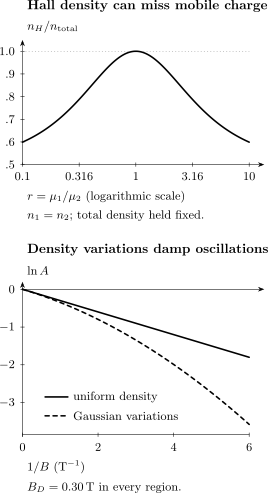
Two ways a fitted quantity can differ from the underlying one. Top: two equal electron populations give $n_H=n_{\rm total}$ only at equal mobility. Bottom: Gaussian frequency variations bend a Dingle plot even though every region has the same $B_D=0.30\,\mathrm T$. The dashed curve uses $\sigma_F=0.05\,\mathrm T$; the solid curve has uniform density. Both amplitudes have been divided by the thermal factor and common prefactor.

The Onsager relation for a resolved closed orbit of area $A_F$ is

$$F=\frac{\hbar A_F}{2\pi e}.$$

For a filled electron pocket with multiplicity $g$, this gives $n_s=geF/h$. Resolved spin or valley pockets must be counted separately. Low-mobility carriers can contribute charge and Hall response while producing no visible oscillation frequency.

Measurement	What it constrains
Sheet conductance	Mobility-weighted carrier density
Low-field Hall slope	Density weighted by squared mobilities
Oscillation frequencies	Areas of visible closed orbits
Dingle damping	Broadening plus possible averaging
Capacitance	Charge response, including electrostatics and traps
Depth-sensitive probes	Extent of the carrier distribution

The measurements become more informative together. For example, compare a gate-induced charge change with the changes in all resolved orbit areas before assigning a new Hall slope to a new subband.

From oscillations to quantum Hall states

For positive $B$, the total filling factor and magnetic length are

$$\nu=\frac{n_s h}{eB}, \qquad \ell_B=\sqrt{\frac{\hbar}{eB}}.$$

Resolving orbital quantization needs sufficiently small $k_{\mathrm B}T$ and $\Gamma_q$ relative to $\hbar\omega_c$, as the damping factors quantify. The classical criterion $\omega_c\tau_{\rm tr}\gtrsim1$ alone is insufficient. Finite-width integer Hall plateaus additionally involve localization; fractional Hall states require the relevant interaction gap to survive disorder and temperature. High mobility alone guarantees neither effect.

Spin–orbit coupling can change the occupied region

Structural inversion asymmetry permits

$$H_R=\alpha(\sigma_xk_y-\sigma_yk_x).$$

For a parabolic band with this Rashba term, define

$$k_R=\frac{m^*|\alpha|}{\hbar^2}, \qquad E_R=\frac{\hbar^2k_R^2}{2m^*}.$$

The lower branch is

$$E_-(k)=\frac{\hbar^2(k-k_R)^2}{2m^*}-E_R.$$

Its minimum is a circle. For $-E_R<\mu<0$, only this branch is occupied, in an annulus between $k_{\rm in}=k_R-q$ and $k_{\rm out}=k_R+q$, where

$$q=\frac{\sqrt{2m^*(\mu+E_R)}}{\hbar}.$$

Both contours belong to the same helicity branch. Their occupied area gives

$$n_s=\frac{k_{\rm out}^2-k_{\rm in}^2}{4\pi} =\frac{k_Rq}{\pi}.$$

When two independent semiclassical orbits are resolved, the density is $e(F_{\rm out}-F_{\rm in})/h$, not the sum of their frequencies. For $\mu>0$, the two helicity branches instead form two occupied disks. Thus two frequencies alone do not establish two confinement subbands or two oppositely split spin populations. Magnetic breakdown, Zeeman coupling and the accessible field range can further complicate the oscillation pattern (Bychkov and Rashba, 1984).

Gating changes confinement, density and scattering as well as spin–orbit coupling. The symmetry and spin textures, including Dresselhaus terms, are developed in Spin–Orbit Coupling in Solids.

Oxide interfaces require an orbital and electrostatic model

The conducting LaAlO$_3$/SrTiO$_3$ interface showed that two insulating oxides can support mobile interface electrons (Ohtomo and Hwang, 2004). Several Ti-derived orbitals, anisotropic masses and a strongly field-dependent dielectric response can participate. A single parabolic band with a fixed dielectric constant is therefore a model to test, not a universal description.

Polar discontinuity, oxygen vacancies, intermixing, surface chemistry and electrostatic gates can contribute jointly to charge redistribution (Zubko and colleagues, 2011). Formal compensation charge need not equal mobile Hall charge. Depth-sensitive measurements, field-angle dependence, oxygen annealing and independently constrained multiband transport help distinguish a confined electron system from conduction extending into the substrate. Engineered Heterostructures develops this interface comparison further.

Exercises

1. Fermi and transport scales. For the GaAs-like example above, calculate $k_F$, $v_F$, $\tau_{\rm tr}$ and $\ell_{\rm tr}$. Does the mobility determine $\tau_q$?

Solution

Convert the density to $3.0\times10^{15}\,\mathrm m^{-2}$ and mobility to $100\,\mathrm{m^2/(V\,s)}$. Then

$$\begin{aligned} k_F&=\sqrt{2\pi n_s}\\ &=1.37\times10^8\,\mathrm m^{-1}, \end{aligned}$$ $$v_F=\frac{\hbar k_F}{0.067m_e} =2.37\times10^5\,\mathrm{m/s},$$ $$\tau_{\rm tr}=\frac{m^*\mu_{\rm mob}}e=38.1\,\mathrm{ps},$$

and $\ell_{\rm tr}=9.04\,\mu\mathrm m$. The angular scattering distribution is needed to connect $\tau_{\rm tr}$ with $\tau_q$; mobility alone does not provide it.

2. Mean depth and width. Normalize the Fang–Howard probability density and derive its mean and variance. Evaluate $\mathcal F(b)$ and the large-$q$ limit.

Solution

Using $\int_0^\infty z^n e^{-bz}dz=n!/b^{n+1}$ gives

$$\int p(z)dz=1,$$ $$\langle z\rangle=\frac3b,\qquad \langle z^2\rangle=\frac{12}{b^2}.$$

Hence the variance is $3/b^2$ and the width is $\sqrt3/b$. The form factor is $\mathcal F(b)=5/16$, while $\mathcal F(q)\sim3b/(8q)$ at large $q$. Treating the mean depth as a root-mean-square width would overestimate the latter by $\sqrt3$.

3. A misleading Dingle slope. Fit a straight secant to the dashed curve between $1/B=2$ and $6\,\mathrm T^{-1}$. What $B_D$ would the fit infer, and by what factor would it misestimate $\tau_q$?

Solution

Write $x=1/B$ and $c=2\pi^2\sigma_F^2$. The secant slope of $-B_Dx-cx^2$ between $x_1$ and $x_2$ is $-B_D-c(x_1+x_2)$. Thus

$$c=2\pi^2\sigma_F^2=0.04935\,\mathrm T^2,$$ $$B_D^{\rm fit}=0.30\,\mathrm T+c(8\,\mathrm T^{-1})$$

gives $B_D^{\rm fit}=0.695\,\mathrm T$. Since $\tau_q\propto1/B_D$,

$$\frac{\tau_q^{\rm fit}}{\tau_q}=\frac{0.30}{0.695}=0.432.$$

The inferred lifetime is less than half the local lifetime, even though no extra scattering was introduced.

4. Hall density at fixed charge. Derive the two-population curve. Check its value at equal mobility and its extreme-mobility limit.

Solution

For $n_1=n_2=n_0$, substitution gives

$$n_H=n_0\frac{(\mu_1+\mu_2)^2}{\mu_1^2+\mu_2^2}.$$

Dividing by $n_{\rm total}=2n_0$ gives the plotted expression. It equals one at $r=1$ and tends to $1/2$ as either population becomes much more mobile. The more mobile carriers dominate the Hall response while the other half of the total charge remains present.

5. Count an annulus. Independent orbit areas in the lower Rashba branch correspond to $F_{\rm out}=8\,\mathrm T$ and $F_{\rm in}=2\,\mathrm T$. Find the sheet density and explain why there is no factor of two.

Solution

Subtract the empty inner disk from the outer disk:

$$\begin{aligned} n_s&=\frac{e(8-2)\,\mathrm T}{h}\\ &=1.45\times10^{11}\,\mathrm{cm}^{-2}. \end{aligned}$$

Each momentum has one occupied helicity state, so there is no unresolved spin multiplicity. Summing the frequencies would instead give $2.42\times10^{11}\,\mathrm{cm}^{-2}$, counting the central empty region incorrectly.

References

• T. Ando, A. B. Fowler and F. Stern, “Electronic Properties of Two-Dimensional Systems,” Reviews of Modern Physics 54, 437–672 (1982), doi:10.1103/RevModPhys.54.437.
• Yu. A. Bychkov and E. I. Rashba, “Oscillatory Effects and the Magnetic Susceptibility of Carriers in Inversion Layers,” Journal of Physics C: Solid State Physics 17, 6039–6045 (1984), doi:10.1088/0022-3719/17/33/015, author-hosted paper.
• P. T. Coleridge, “Small-Angle Scattering in Two-Dimensional Electron Gases,” Physical Review B 44, 3793–3801 (1991), doi:10.1103/PhysRevB.44.3793.
• F. F. Fang and W. E. Howard, “Negative Field-Effect Mobility on (100) Si Surfaces,” Physical Review Letters 16, 797–799 (1966), doi:10.1103/PhysRevLett.16.797.
• A. Ohtomo and H. Y. Hwang, “A High-Mobility Electron Gas at the LaAlO$_3$/SrTiO$_3$ Heterointerface,” Nature 427, 423–426 (2004), doi:10.1038/nature02308.
• F. Stern, “Polarizability of a Two-Dimensional Electron Gas,” Physical Review Letters 18, 546–548 (1967), doi:10.1103/PhysRevLett.18.546.
• P. Zubko, S. Gariglio, M. Gabay, P. Ghosez and J.-M. Triscone, “Interface Physics in Complex Oxide Heterostructures,” Annual Review of Condensed Matter Physics 2, 141–165 (2011), doi:10.1146/annurev-conmatphys-062910-140445.