Quantum Wells

A quantum well confines motion in one direction and leaves two directions extended. Each bound transverse level becomes the bottom of a two-dimensional subband. Confinement determines which states exist; carrier density determines which are occupied; the probe and broadening determine which features can be resolved.

A populated well can support a Two-Dimensional Electron Gas, while an optical well can have empty conduction subbands before illumination. This page develops the confinement, interface conditions and optical transitions needed to understand both cases.

Required background. Effective Mass supplies the band-edge approximation, Finite Square Well supplies bound-state matching, and Fermi–Dirac Statistics supplies occupations.

Confinement and subbands in a quantum well

Let $z$ be the growth direction. For an isolated conduction band, a common envelope Hamiltonian is

$$H_z=-\frac{\hbar^2}{2}\partial_z\frac{1}{m_z(z)}\partial_z+V(z).$$

The envelope $\chi_n$ varies over distances larger than a unit cell; the microscopic Bloch function supplies the underlying band character. Solve $H_z\chi_n=\varepsilon_n\chi_n$ with normalized bound states. If the in-plane mass is constant and isotropic,

$$E_n(\mathbf k_\parallel)=\varepsilon_n+\frac{\hbar^2k_\parallel^2}{2m_\parallel}.$$

The envelope then does not depend on in-plane momentum. Merely adding in-plane energy above another threshold does not automatically transfer an electron to another subband: scattering, preparation and equilibrium occupation determine that transfer.

If $m_\parallel$ varies across the structure, the term $\hbar^2k_\parallel^2/[2m_\parallel(z)]$ changes the transverse eigenproblem itself. For an isolated subband near $k_\parallel=0$, perturbation theory gives

$$\frac{1}{m_{\parallel,n}}= \int dz\,\frac{|\chi_n(z)|^2}{m_\parallel(z)}.$$

Higher orders mix envelopes and can produce nonparabolic dispersion. An average inverse mass is a leading small-momentum approximation, not an exact separation for arbitrary in-plane energy.

At zero temperature only the lowest subband is occupied when $\varepsilon_1<\mu<\varepsilon_2$. At finite temperature the second subband has a thermal tail rather than an abrupt empty/full boundary. Resolving thresholds additionally requires sufficiently narrow instrumental and physical linewidths. These conditions do not guarantee long in-plane phase coherence. Quantum Coherence in Conductors explains that independent question.

Interface matching conserves probability flux

For the displayed Hamiltonian, a finite abrupt mass/potential step without a singular interface term requires continuity of

$$\chi,\qquad \frac{1}{m_z}\partial_z\chi.$$

Integrating the differential equation across the step gives the second condition. The first belongs to the finite-energy domain of this divergence-form operator. Together they conserve

$$j_z=\hbar\,\operatorname{Im} \left(\chi^*\frac{1}{m_z}\partial_z\chi\right).$$

These are the BenDaniel–Duke conditions. Matching the ordinary derivative across unequal masses generally fails to conserve current. Current continuity alone, however, does not determine a unique interface model: interface potentials or other self-adjoint matching conditions can conserve flux too. The stated conditions follow from the stated Hamiltonian (BenDaniel and Duke).

This one-band approximation needs care at atomically abrupt interfaces. Valley coupling, interface-specific terms, nonparabolicity and especially heavy/light-hole mixing may require multiband or microscopic models. The matching rules must follow that model rather than being carried over unchanged.

A finite barrier changes both energies and wavefunctions

For a well of width $L$ with impenetrable walls and constant interior mass $m_w$,

$$\varepsilon_n^{(\infty)}=\frac{\hbar^2\pi^2n^2}{2m_wL^2}.$$

At $L=10\,\mathrm{nm}$ and $m_w=0.067m_e$, the first three values are approximately $56.1$, $224.5$ and $505.1\,\mathrm{meV}$ relative to the well bottom. The $L^{-2}$ scaling is useful, but an infinite wall cannot predict leakage or the number of finite-well bound states.

For an illustrative symmetric finite well, use the same width and interior mass, barrier mass $m_b=0.091m_e$ and height $V_0=300\,\mathrm{meV}$. With $a=L/2$, define

$$k=\frac{\sqrt{2m_wE}}{\hbar},$$ $$\kappa=\frac{\sqrt{2m_b(V_0-E)}}{\hbar}.$$

For even and odd envelopes respectively, matching gives

$$\frac{k}{m_w}\tan(ka)=\frac{\kappa}{m_b},$$ $$-\frac{k}{m_w}\cot(ka)=\frac{\kappa}{m_b}.$$

There are three bound levels: approximately $32.08$, $126.53$ and $267.76\,\mathrm{meV}$. The third exists even though the third infinite-well energy exceeds the barrier. Truncating the infinite ladder at $V_0$ therefore gives the wrong state count. Barrier penetration lowers energies; its extent grows for weakly bound states. The parameters define a model, not a complete prediction for an alloy sample.

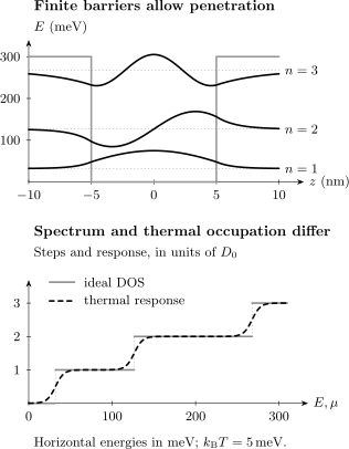
Top: the three bound envelopes for the stated finite well, shifted vertically to their energies and scaled for visibility. Their tails continue into the barriers. Bottom: taking one common constant in-plane mass, each bound subband contributes a sharp density-of-states step $D_0$. The dashed curve instead shows $(\partial n_s/\partial\mu)/D_0$ at $k_{\rm B}T=5\,\mathrm{meV}$. Temperature rounds this occupation response while the fixed noninteracting spectrum remains unchanged. Only contributions from these bound subbands are shown.

Two-dimensional state counting and occupation

One state per internal component occupies area $(2\pi)^2/A$ in the in-plane momentum plane. An isotropic parabolic subband therefore contains

$$\frac{N_n(E)}{A}=\frac{g_n k^2}{4\pi}$$

states below energy $E>\varepsilon_n$. Here $g_n$ counts degenerate spin/valley states, not the two signs of momentum. Define the density of states per area as $D(E)$ and write

$$D(E)=\sum_n D_n\Theta(E-\varepsilon_n),$$ $$D_n=\frac{g_nm_{\parallel,n}}{2\pi\hbar^2}.$$

For an elliptical parabola use $m_{\rm DOS}=\sqrt{m_xm_y}$. Its perpendicular-field cyclotron mass equals that geometric mean, while directional transport retains the separate masses. These identities depend on the elliptical parabolic model; see Effective Mass.

Integrating against the Fermi function gives

$$n_s=\sum_n D_n k_{\rm B}T\ln(1+e^{\eta_n}),$$ $$\eta_n=\frac{\mu-\varepsilon_n}{k_{\rm B}T}.$$

At zero temperature this reduces to $\sum_nD_n(\mu-\varepsilon_n)\Theta(\mu-\varepsilon_n)$. At fixed spectrum the thermal density response is

$$\frac{\partial n_s}{\partial\mu} =\sum_n\frac{D_n}{1+e^{-\eta_n}}.$$

This response is smooth even though $D(E)$ is still a staircase. Temperature alone does not broaden the density of states of a fixed noninteracting Hamiltonian. Temperature-dependent scattering, interactions or structural changes can alter the actual spectrum, and measurement convolutions can smooth its appearance. Thermodynamic compressibility, tunneling spectra and optical absorption also involve different responses.

For one GaAs-like subband with $m_\parallel=0.067m_e$, $g=2$ and $\mu-\varepsilon_1=10\,\mathrm{meV}$, the zero-temperature density is $2.80\times10^{11}\,\mathrm{cm}^{-2}$. Comparing that Fermi energy with the next threshold tests single-subband occupation. Quantum Wires derives the one-dimensional singularity; Quantum Dots treats fully discrete spectra.

Band offsets and self-consistent confinement

A heterostructure barrier is a conduction- or valence-band offset, not the full bulk band gap. Strain, composition, electrostatic fields and interface chemistry can change it. Quantitative material parameters must match the intended structure; Vurgaftman, Meyer and Ram-Mohan provide a widely used III–V compilation.

Band alignment	Carrier arrangement
Type I: straddling	Electron and hole confinement favor the same material
Type II: staggered	Electron and hole confinement favor different layers
Type III: broken gap	A conduction edge lies below the other material’s valence edge

Type I permits strong optical overlap but does not guarantee it. Type II can reduce overlap; fields and tunneling still matter. Broken-gap structures require attention to charge transfer and electron–hole hybridization.

Mobile charge reshapes the confinement. A minimal Schrödinger–Poisson calculation iterates

$$\partial_z[\epsilon(z)\partial_z\phi]=-\rho(z),$$

with electron potential $V=V_{\rm band}-e\phi$ and density

$$n(z)=\sum_n n_{s,n}|\chi_n(z)|^2.$$

Include dopants, fixed interface and polarization charges, and the gates’ boundary conditions. An exchange-correlation potential is an additional approximation. Isolated devices require an appropriate total-charge constraint; gated devices can carry net layer charge balanced elsewhere. Arbitrarily increasing the density in a fixed empty-well potential misses this feedback (Ando, Fowler and Stern).

Neighboring wells also hybridize. Coupled Wells and Avoided Crossings derives the tunnel splitting; periodic arrays form minibands. Resonant Transmission treats the corresponding open scattering problem. These are extensions of confinement, not additional universal square-well formulas.

Optical transitions require the right matrix element

Interband transitions and excitons

An interband transition creates an electron–hole pair. A simple continuum threshold is $E_g+\varepsilon_{e,n}+\varepsilon_{h,m}$; attraction can bind an exciton below the matching continuum. Bloch dipole elements, polarization and envelope overlap determine which states are bright. The envelope factor is

$$\mathcal O_{nm}=\int dz\,\chi_{e,n}^*\chi_{h,m}.$$

The rule $n=m$ follows exactly when the two sets have the same orthonormal envelope functions, as in the ideal hard-wall model even with different constant masses. For different finite barriers, electron and hole eigenfunctions are not one common orthogonal basis. Equal parity can then allow overlap between different indices; opposite parity still forbids it in an ideal symmetric structure. Hole-band mixing and broken symmetry add further qualifications.

Photoluminescence additionally depends on carrier relaxation and populations. A line below a calculated independent-particle threshold can reflect an exciton, localization, a changed gap or an inaccurate confinement model. Compare absorption and emission before assigning their difference to binding energy.

Intersubband polarization and parity

An electron within one band couples through the growth-direction dipole

$$z_{nm}=\int dz\,\chi_n^*z\chi_m.$$

An ideal normally incident plane wave on an unpatterned layer has no growth-direction electric field, so it cannot drive this transition in the one-band dipole approximation. Oblique incidence, waveguides or patterned coupling can supply that component (Helm).

In a symmetric well, $z$ connects opposite-parity states. This does not impose $\Delta n=1$. In a hard-wall well on $0<z<L$, distinct opposite-parity levels have

$$z_{nm}=-\frac{8Lnm}{\pi^2(n^2-m^2)^2}.$$

Thus $1\to4$ is allowed as well as $1\to2$, while $1\to3$ vanishes. With constant mass, the dimensionless oscillator strength is

$$f_{1m}=\frac{2m_z}{\hbar^2} (\varepsilon_m-\varepsilon_1)|z_{1m}|^2.$$

For the infinite well, $f_{12}\simeq0.9607$ and $f_{14}\simeq0.03074$. The first transition dominates, but the others are not prohibited. Finite barriers add continuum transitions, and interacting populated wells can show collective depolarization shifts; a measured line need not equal a bare level difference.

The quantum-confined Stark effect

A field $F$ along $z$ adds $eFz$ to an electron’s potential and the opposite sign for a hole. In a centered symmetric well, the first-order shift of a nondegenerate ground state vanishes. Its leading shift is

$$\delta\varepsilon_1^{(2)}=(eF)^2 S_1,$$ $$S_1=\sum_{m\ne1}\frac{|z_{1m}|^2}{\varepsilon_1-\varepsilon_m},$$

which is negative when the complete discrete/continuum sum is taken. Electron and hole envelopes shift in opposite directions, usually reducing their overlap. This explains the basic redshift of a symmetric type-I well before strong escape, screening and changes in binding become dominant (Miller and colleagues).

Built-in fields change the reference: an applied field that cancels an existing tilt can increase overlap and shift a transition upward. A universal redshift for every applied-field direction is therefore not a selection rule. Semiconductor Lasers Overview connects these optical transitions to gain and cavities.

Exercises

1. Count finite-well levels

For the finite well above, the maximum interior phase is $k_{max}a\simeq3.63$. Explain why three bound states are possible even though only two infinite-well levels lie below $V_0$.

Solution

The even matching equation has roots in $0<ka<\pi/2$ and $\pi<ka<3.63$; the odd equation has one in $\pi/2<ka<\pi$. Penetration relaxes the hard-wall constraint, so the third finite-well state moves below the barrier. Counting infinite-well energies below $V_0$ omits that state. A solution exactly at the exterior continuum threshold is not a square-integrable bound state.

2. Reflection from a mass step

At equal potential on both sides, let $m_R=4m_L$. For an incident energy above that potential, use $r=(v_L-v_R)/(v_L+v_R)$ and $t=1+r$ to calculate reflection and transmitted flux.

Solution

Since $v\propto m^{-1/2}$ at fixed kinetic energy, $v_R=v_L/2$. Thus $r=1/3$ and $t=4/3$. The probabilities are

$$R=|r|^2=\frac19,$$ $$T=\frac{v_R}{v_L}|t|^2=\frac89.$$

They sum to one. The amplitude $t$ can exceed one because transmitted flux also includes the group velocity. Matching the ordinary derivative would give the wrong velocity weighting for this Hamiltonian.

3. How weak is the allowed 1-to-4 line?

Use the hard-wall energies and dipole elements to compute $f_{14}/f_{12}$.

Solution

The dipole ratio is $|z_{14}/z_{12}|=0.08$, but oscillator strength also weights the transition energy. Therefore

$$\frac{f_{14}}{f_{12}}=\frac{15}{3}(0.08)^2=0.032.$$

The higher line has about $3.2\%$ of the first line’s oscillator strength in this model. Symmetry allows it; the matrix element makes it weaker.

4. A thermally occupied second subband

For equal step heights, take $\mu-\varepsilon_1=10\,\mathrm{meV}$, $\varepsilon_2-\varepsilon_1=30\,\mathrm{meV}$ and $k_{\rm B}T=5\,\mathrm{meV}$. Find $n_{s,2}/n_{s,1}$ and state whether the underlying fixed-spectrum DOS is rounded.

Solution

$$\frac{n_{s,2}}{n_{s,1}} =\frac{\ln(1+e^{-4})}{\ln(1+e^2)} \simeq0.00853.$$

The second subband has about $0.85\%$ of the first one’s density. Its occupation is small, not exactly zero. The ideal fixed-spectrum DOS keeps its steps; Fermi weighting smooths occupation and the density response.

5. Symmetry versus equal subband indices

Electron and hole potentials are both symmetric but have different finite barrier heights. Is the interband envelope overlap between their first and third levels necessarily zero? Compare with the first-to-second overlap.

Solution

The first and third envelopes are even, so their product is even and symmetry does not force the overlap to vanish. They belong to different eigenproblems, so orthogonality within either one does not prove cross-orthogonality. The first-to-second product is odd and integrates to zero in the symmetric model. Identical envelope bases would additionally enforce equal indices; asymmetry removes even the parity argument.

References

• T. Ando, A. B. Fowler, and F. Stern, “Electronic Properties of Two-Dimensional Systems,” Reviews of Modern Physics 54, 437–672 (1982), doi:10.1103/RevModPhys.54.437.
• D. J. BenDaniel and C. B. Duke, “Space-Charge Effects on Electron Tunneling,” Physical Review 152, 683–692 (1966), doi:10.1103/PhysRev.152.683.
• M. Helm, “The Basic Physics of Intersubband Transitions,” in H. C. Liu and F. Capasso (eds.), Intersubband Transitions in Quantum Wells: Physics and Device Applications I, Semiconductors and Semimetals 62, Academic Press, 1–99 (2000), publisher chapter.
• D. A. B. Miller, D. S. Chemla, T. C. Damen, A. C. Gossard, W. Wiegmann, T. H. Wood, and C. A. Burrus, “Band-Edge Electroabsorption in Quantum Well Structures: The Quantum-Confined Stark Effect,” Physical Review Letters 53, 2173–2176 (1984), doi:10.1103/PhysRevLett.53.2173.
• I. Vurgaftman, J. R. Meyer, and L. R. Ram-Mohan, “Band Parameters for III–V Compound Semiconductors and Their Alloys,” Journal of Applied Physics 89, 5815–5875 (2001), doi:10.1063/1.1368156.

Further reading

• G. Bastard, Wave Mechanics Applied to Semiconductor Heterostructures, Les Éditions de Physique (1988).
• J. H. Davies, The Physics of Low-Dimensional Semiconductors, Cambridge University Press (1998), doi:10.1017/CBO9780511819070.