Quantum Dots

A quantum dot confines carriers in all spatial directions, producing discrete localized orbitals. Its electrical spectrum asks how much energy it takes to add or remove an electron; its optical spectrum asks how much energy a radiative transition releases. Neither is generally a list of bare orbital energies.

The phrase artificial atom captures shell filling and discrete transitions, but the confinement, screening and tunnel contacts are engineered. This page develops the connection between confinement and measured spectra. Coulomb Blockade derives junction energetics and diamond slopes; Mesoscopic Transport develops the general rate equations.

Required background. Finite Square Well explains localized levels and leakage. Chemical Potential explains addition energies and reservoir equilibrium; Fermions supplies Pauli filling. Mesoscopic Transport supplies the tunneling probabilities used below.

Confined orbitals and resolved spectra

Zero-dimensional describes the absence of an extended propagation direction in the localized spectrum, not a point of zero size or a requirement that only one level be occupied. Finite confinement also permits continuum states above escape thresholds. Coupling a localized level to leads turns it into a resonance.

Gate-defined semiconductor dots use electrostatic barriers; etched structures and nanowires add material boundaries. Epitaxial dots use strain and band offsets, while colloidal nanocrystals add dielectric interfaces and surface chemistry. Metallic islands can show charge quantization even when their dense orbital spectrum is unresolved. The measurement’s energy resolution decides whether individual orbitals must be retained.

For a simple semiconductor model, define each electron’s kinetic momentum $\boldsymbol\pi_i=\mathbf p_i+e\mathbf A(\mathbf r_i)$, with electron charge $-e$. Then

$$H_{\rm dot}=\sum_i h_i+\sum_{i<j}V_{ij},$$ $$h_i=\frac{\boldsymbol\pi_i^2}{2m^*}+V_{\rm conf}(\mathbf r_i) +H_{{\rm SO},i}+H_{Z,i}.$$

The screened interaction $V_{ij}$, effective mass, spin–orbit coupling and Zeeman term depend on the material and geometry. A gate voltage is an electrostatic boundary condition; solving the device electrostatics gives the actual confinement potential.

A shell benchmark and a spacing convention

For an isotropic two-dimensional harmonic dot at zero field,

$$\epsilon_{n_xn_y}=\hbar\omega_0(n_x+n_y+1).$$

The shell $s=n_x+n_y$ has $s+1$ spatial orbitals. With two degenerate spins, complete shells contain a total of $2,6,12,\ldots$ electrons. This is a benchmark, not a universal filling rule: ellipticity, valley structure, exchange and correlations can change the pattern. Shell and spin effects were resolved in vertical dots by Tarucha and colleagues. The perpendicular-field orbital spectrum is derived in Charged Harmonic Oscillator in a Magnetic Field.

For a large two-dimensional dot of electronic area $A$, the leading smooth density of states gives

$$\overline\Delta_{\rm orb}=\frac{2\pi\hbar^2}{m^*A}.$$

This counts one copy of each spatial orbital. If each orbital has $g$ exactly degenerate internal states, the inverse total density of states is $\overline\Delta_{\rm state}=\overline\Delta_{\rm orb}/g$. It is not the separation between distinct orbital energies: exact partners have zero separation. For $m^*=0.067m_e$ and $A=0.040\,\mu\mathrm m^2$, these estimates are $179\,\mu\mathrm{eV}$ per spatial orbital and $89\,\mu\mathrm{eV}$ per state for $g=2$. Boundary corrections and spectral fluctuations matter in small dots (Alhassid).

Charging, temperature and escape

We use $E_C=e^2/(2C_\Sigma)$ for the charging coefficient. Some literature calls $e^2/C_\Sigma$ the charging energy, so compare definitions before numbers. We use $\Gamma_\alpha$ for an energy width and $\gamma_\alpha=\Gamma_\alpha/\hbar$ for a tunneling rate.

For a wide-band noninteracting resonance with pole $\epsilon_d-i\Gamma/2$, the survival probability decays with time constant $\hbar/\Gamma$, where $\Gamma=\Gamma_L+\Gamma_R$. Interacting many-state transport need not have one common escape time.

Individual levels require thermal and linewidth scales below the relevant separation. Well-defined charge plateaus require weak charge fluctuations and temperature below their addition gap; charge necessarily fluctuates near a degeneracy. The conditions for resolving orbitals and for resolving charge are different. A dense metallic island can satisfy only the latter.

Constant-interaction model

The constant-interaction model retains a fixed spectrum of spin-orbitals $\epsilon_i$ and adds a capacitance energy. Let $n_g$ be the induced charge in units of $e$, including gates, leads and offset charge. With the lowest $N$ spin-orbitals filled,

$$E_N=\sum_{i=1}^N\epsilon_i+E_C(N-n_g)^2.$$

The electrochemical potential for the $N$th electron is a first difference:

$$\mu_N=E_N-E_{N-1},$$ $$\mu_N=\epsilon_N+2E_C(N-\tfrac12-n_g).$$

The separation between consecutive addition thresholds is a second difference:

$$E_{\rm add}(N)=\mu_{N+1}-\mu_N,$$ $$E_{\rm add}(N)=\epsilon_{N+1}-\epsilon_N+2E_C.$$

Thus filling the second spin in one orbital costs the same charging increment but no new orbital spacing. Starting the next shell adds both contributions. For $C_\Sigma=80\,\mathrm{aF}$, $E_C\simeq1.00\,\mathrm{meV}$; an orbital spacing of $0.40\,\mathrm{meV}$ gives $E_{\rm add}\simeq2.40\,\mathrm{meV}$ across that orbital boundary.

A plunger gate with lever arm $\alpha_g=C_g/C_\Sigma$ shifts a transition by $\delta\mu_N=-e\alpha_g\delta V_g$. If the spectrum and capacitances stay fixed, adjacent zero-bias peak positions obey

$$e\alpha_g\Delta V_g=E_{\rm add}(N).$$

The familiar period $e/C_g$ therefore applies when the orbital increment is negligible, not to every pair of peaks. Barrier gates can change both widths and energies; deformation and cross-capacitance invalidate a single constant lever arm over a large sweep.

Exchange and correlation corrections vary between charge sectors. A useful exact statement remains $\mu_N=E_N-E_{N-1}$ for ground-state energies, even when the constant-interaction approximation fails. Excited-state spectroscopy instead involves differences such as $E_{N,a}-E_{N-1,b}$. A large addition energy alone does not identify a shell closure (Kouwenhoven, Austing and Tarucha).

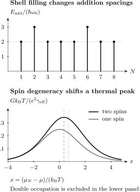
Top: constant-interaction addition spacings for a circular harmonic dot with two spins per orbital and $2E_C=2\hbar\omega_0$. Peaks at $N=2,6$ mark complete shells in this ideal model. Bottom: sequential conductance in units of $e^2\gamma_{\rm eff}/(k_{\rm B}T)$. One allowed spin gives a symmetric peak; two available spins with double occupation excluded shift and reshape it. The dashed vertical line marks the latter conductance maximum, while the dotted line marks equal empty/occupied probabilities. These are different locations.

What a transport peak measures

At low temperature, sequential transport can occur when a transition energy lies between lead chemical potentials. This is necessary but not sufficient: the tunneling matrix element must be nonzero, the initial state must be occupied, and no trapped state may block the cycle. Spin selection rules can suppress energetically allowed transport.

A finite-bias charge-stability plot contains low-current Coulomb diamonds. Their boundaries align a charge transition with a lead; slopes and vertical extent depend on capacitances and the bias convention. Coulomb Blockade derives that conversion. Parallel lines can come from dot excitations, lead structure, phonons or another island, so a line’s appearance alone is not an assignment.

The nondegenerate thermal peak

Consider one empty state and one occupied state, with energy-independent rates, equilibrium leads, and $\Gamma\ll k_{\rm B}T$ well below other addition energies. Define

$$\gamma_{\rm eff}=\frac{\gamma_L\gamma_R}{\gamma_L+\gamma_R},$$

and let $x=(\mu_N-\mu)/(k_{\rm B}T)$. The linear conductance is

$$G=\frac{e^2\gamma_{\rm eff}}{k_{\rm B}T}\,g_1(x),$$ $$g_1(x)=\frac{1}{4\cosh^2(x/2)}.$$

Its energy FWHM is $3.53k_{\rm B}T$. This permits electron thermometry only when lifetime broadening, additional states and temperature-dependent barriers are negligible (Beenakker). Linear response itself requires bias small on the scale over which current changes, commonly $e|V|\ll k_{\rm B}T$ for this peak; being below the much larger addition gap is insufficient.

Two spins change both the peak and the charge crossover

Now allow $|0\rangle$, $|\uparrow\rangle$ and $|\downarrow\rangle$, excluding double occupation by a large repulsion. Assume zero spin splitting, equal rates per spin and no spin polarization. An empty dot has two ways to fill, while an occupied dot has only one electron to emit. For lead $\alpha$ the total filling and emptying rates are

$$a_\alpha=2\gamma_\alpha f_\alpha,$$ $$b_\alpha=\gamma_\alpha(1-f_\alpha).$$

Solving the same population equations gives

$$G=\frac{e^2\gamma_{\rm eff}}{k_{\rm B}T}\,g_2(x),$$ $$g_2(x)=\frac{2f(1-f)}{1+f},$$ $$f=\frac{1}{1+e^x}.$$

The maximum is at $x=\tfrac12\ln2$, not at the bare ground-state degeneracy $x=0$. Equilibrium probabilities instead satisfy $P_1/P_0=2e^{-x}$, so equal charge probabilities occur at $x=\ln2$. The factor of two is the occupied sector’s spin entropy. A conductance maximum, a half-occupation point and a zero-temperature energy crossing need not coincide.

More generally, nearly degenerate charge sectors with multiplicities $d_N$ have a free-energy difference containing $-k_{\rm B}T\ln(d_N/d_{N-1})$. Excited states or unequal couplings require their actual partition functions and rates, not an automatic degeneracy multiplier.

When the thermal peak fails

For $\Gamma\gtrsim k_{\rm B}T$, coherent lifetime broadening matters. Virtual transitions produce cotunneling even inside a sequential-blockade valley. An odd local moment coupled to normal metallic leads can enter the Kondo regime; a zero-bias peak alone does not identify it. Anderson Impurity Model Preview explains the interacting level, and Conductance Quantization treats elastic transmission. Superconducting contacts require Proximity and Andreev Physics.

Spin spectroscopy and coupled dots

Magnetic-field slopes contain both orbital and spin contributions. The Zeeman splitting is $|g^*|\mu_BB$, but a transition measures the difference between initial and final magnetic moments. Valley splitting, exchange, spin–orbit avoided crossings and changing lever arms can complicate a fitted $g$ factor (Hanson and colleagues).

In a double dot, one electron hybridizes between left and right orbitals. With real tunnel amplitude $t_c$ and detuning $\varepsilon$,

$$H=\frac{\varepsilon}{2}\sigma_z+t_c\sigma_x,$$ $$\Delta E=\sqrt{\varepsilon^2+4t_c^2}.$$

At zero detuning the eigenstates are equally shared between the dots and the splitting is first-order insensitive to detuning. Tunnel-amplitude noise still changes it linearly, and second-order detuning noise remains. Charge hybridization does not by itself imply greater sensitivity to every noise direction. The algebra is in Tight-Binding Dimer; the transport setting is reviewed by van der Wiel and colleagues.

Spin-selective tunneling and Pauli spin blockade can convert spin into charge information. Quantum Point Contacts explains charge sensing; Spin Qubits and Silicon Spin Qubits develop control, leakage and readout. A Coulomb valley or an avoided crossing alone does not demonstrate a working qubit.

Optical transitions compare many-body states

Optical excitation creates an electron–hole pair. A minimal neutral-exciton estimate is

$$E_X=E_g+\epsilon_e+\epsilon_h-U_{eh},$$

where $U_{eh}>0$ denotes attraction. Exchange, strain, dielectric mismatch, fine structure and configuration mixing refine this model. For a neutral exciton recombining to the empty dot, the photon carries $E_X$ relative to that empty reference. A charged exciton leaves a carrier behind, whose energy must be subtracted:

$$\hbar\omega=E_{\rm initial}-E_{\rm final}.$$

Consequently, photoluminescence cannot be read as one electron’s orbital or electrical addition energy. Polarization, charge tuning, power dependence and photon correlations help distinguish exciton complexes (Warburton). Spontaneous Emission and Antibunching develop the optical diagnostics.

Measurement	Physical quantity and main qualification
Linear conductance	Transition rates and occupations; not only energy alignment
Finite-bias lines	Many-body transitions after electrostatic conversion
Charge sensing	Occupation changes, including states carrying little current
Magnetospectroscopy	Differences of orbital and spin moments
Optical emission	Radiative initial-to-final energy differences

For transport dots, compare charge sensing with current to identify suppressed transitions. For optical dots, compare charge tuning with emitted-photon statistics. Single-Electron Devices develops controlled transfer, while Nanostructures for Quantum Technology connects confinement to device performance.

Exercises

1. Distinct orbitals or individual states?

A dot’s inverse total density of states is $89\,\mu\mathrm{eV}$ with two exactly degenerate spins per spatial orbital. What is the mean distinct-orbital spacing? Does resolving the $89\,\mu\mathrm{eV}$ scale resolve the spin partners?

Solution

The spatial-orbital estimate is twice as large, about $178\,\mu\mathrm{eV}$ (the unrounded area estimate above gives $179\,\mu\mathrm{eV}$). Exact spin partners remain degenerate regardless of spectroscopic resolution. Resolving separate spin lines requires a physical splitting, not just a narrower measurement.

2. Addition peaks across a shell

For $C_\Sigma=80\,\mathrm{aF}$ and $C_g=8\,\mathrm{aF}$, compare gate spacings when the next spin-orbital increment is zero and when it is $0.40\,\mathrm{meV}$.

Solution

The lever arm is $0.10$, and the charging increment is $e^2/C_\Sigma\simeq2.00\,\mathrm{meV}$. The addition energies are $2.00$ and $2.40\,\mathrm{meV}$, giving approximately $20.0$ and $24.0\,\mathrm{mV}$ gate spacings. The simple period $e/C_g$ describes only the first case under these assumptions.

3. Where is the spin-degenerate peak?

Write $g_2(x)$ in terms of $y=e^x$ and find its maximum. Compare with the point where the empty and occupied probabilities are equal.

Solution

The shape becomes

$$g_2=\frac{2y}{(1+y)(2+y)}.$$

Its derivative has the sign of $2-y^2$, so the maximum is at $y=\sqrt2$, or $x=\tfrac12\ln2$. The value is $2/(3+2\sqrt2)\simeq0.3431$ in the plotted units. Equal occupation instead requires $2e^{-x}=1$, hence $x=\ln2$. Both shifts vanish in energy units as $T\to0$, although the sequential regime must remain valid when taking that limit.

4. A sweet spot for one noise direction

Expand the double-dot splitting at small $|\varepsilon/t_c|$ with $t_c\ne0$. Identify its leading response to detuning and to a small change in $|t_c|$.

Solution

$$\Delta E=2|t_c|+\frac{\varepsilon^2}{4|t_c|} +O(\varepsilon^4/|t_c|^3).$$

Detuning has no linear term, but the derivative with respect to $|t_c|$ at zero detuning is $2$. A gate-noise direction that changes both parameters is therefore not automatically protected.

5. A charged exciton leaves an electron

In the minimal model, a negative trion has two electrons in one spatial orbital and one hole. Its initial energy is

$$E_{X^-}=E_g+2\epsilon_e+\epsilon_h +U_{ee}-2U_{eh}.$$

Recombination leaves one electron of energy $\epsilon_e$. Find the shift of the trion photon relative to the neutral-exciton photon.

Solution

Subtracting the final electron energy and then $E_X$ gives

$$\hbar\omega_{X^-}-\hbar\omega_X=U_{ee}-U_{eh}.$$

The remaining electron’s one-particle energy cancels; the shift compares repulsion with attraction. It need not equal an electron addition energy or have a universal sign. Relaxed orbitals and correlations modify this deliberately minimal example.

References

• Y. Alhassid, “The Statistical Theory of Quantum Dots,” Reviews of Modern Physics 72, 895–968 (2000), doi:10.1103/RevModPhys.72.895.
• C. W. J. Beenakker, “Theory of Coulomb-Blockade Oscillations in the Conductance of a Quantum Dot,” Physical Review B 44, 1646–1656 (1991), doi:10.1103/PhysRevB.44.1646.
• R. Hanson, L. P. Kouwenhoven, J. R. Petta, S. Tarucha, and L. M. K. Vandersypen, “Spins in Few-Electron Quantum Dots,” Reviews of Modern Physics 79, 1217–1265 (2007), doi:10.1103/RevModPhys.79.1217.
• L. P. Kouwenhoven, D. G. Austing, and S. Tarucha, “Few-Electron Quantum Dots,” Reports on Progress in Physics 64, 701–736 (2001), doi:10.1088/0034-4885/64/6/201.
• S. Tarucha, D. G. Austing, T. Honda, R. J. van der Hage, and L. P. Kouwenhoven, “Shell Filling and Spin Effects in a Few Electron Quantum Dot,” Physical Review Letters 77, 3613–3616 (1996), doi:10.1103/PhysRevLett.77.3613.
• W. G. van der Wiel, S. De Franceschi, J. M. Elzerman, T. Fujisawa, S. Tarucha, and L. P. Kouwenhoven, “Electron Transport through Double Quantum Dots,” Reviews of Modern Physics 75, 1–22 (2002), doi:10.1103/RevModPhys.75.1.
• R. J. Warburton, “Single Spins in Self-Assembled Quantum Dots,” Nature Materials 12, 483–493 (2013), doi:10.1038/nmat3585.

Further reading

• T. Ihn, Semiconductor Nanostructures: Quantum States and Electronic Transport, Oxford University Press (2010), doi:10.1093/acprof:oso/9780199534425.001.0001.