Silicon Spin Qubits

Silicon spin qubits store information in confined electron or nuclear spins. Gate voltages control confinement and exchange; magnetic or electric drives rotate spins; spin-to-charge conversion makes their state measurable. The central tradeoff is that electrical coupling enables useful operations while also exposing a nominally magnetic degree of freedom to charge noise.

A single-electron qubit, a singlet–triplet encoding, a three-spin encoding, and a donor nuclear register use different Hilbert spaces and controls. This page derives their basic gate models and connects them to loading, readout, transport, temperature, and fabrication. Current experimental milestones are discussed in Quantum Hardware Scaling.

Required background. Hardware Overview introduces the preparation–control–measurement cycle; Bits, Qubits, Qudits, and Modes supplies the qubit and subspace language. Spin in Magnetic Fields explains Zeeman splitting, and Quantum Dots develops confinement and addition energies.

From Silicon to a Spin Hamiltonian

Gate-defined quantum dots

In a silicon metal–oxide–semiconductor device, positive gate voltages can accumulate electrons near a Si–SiO₂ interface while barrier gates control tunneling between neighboring regions and reservoirs. In a Si/SiGe device, a strained silicon quantum well confines the carriers vertically and patterned surface gates confine them laterally. In either case, the low-energy dot is an engineered potential minimum, not an isolated atom.

The useful one-electron regime requires several scales to be resolved:

$$E_C,\ \Delta_{\mathrm{orb}},\ \Delta_v \gg k_BT,\ \hbar\Omega,\ \hbar\Gamma,$$

where $E_C$ is a charging scale, $\Delta_{\mathrm{orb}}$ an orbital gap, $\Delta_v$ a valley splitting, $\Omega$ a driven rate, and $\Gamma$ a reservoir or sensor-induced rate. This is a design hierarchy, not a universal ordering. During initialization or readout, one deliberately changes tunnel rates and level alignments; during a fast gate, drive bandwidth may approach some unwanted splitting. Even a large valley gap is insufficient near a spin–valley resonance $E_Z\approx\Delta_v$: the relevant separation is the gap from the driven qubit levels to the unwanted states, not $\Delta_v$ alone.

Silicon has conduction-band valleys. Confinement and interfaces lift their degeneracy, but the resulting $\Delta_v$ depends on electric field, quantum well structure, interface steps, alloy disorder, and dot position. A valley excitation is not merely a higher copy of the qubit. It can hybridize with spin and orbital states, alter exchange, create relaxation hot spots, or provide a leakage channel.

Donors in silicon

A substitutional donor such as phosphorus contributes an electron whose orbital is bound by the impurity potential. The donor nucleus also carries a spin. A minimal electron–nuclear Hamiltonian is

$$H = g_e\mu_B\mathbf B\cdot\mathbf S - g_n\mu_N\mathbf B\cdot\mathbf I + A\,\mathbf S\cdot\mathbf I.$$

Here $\mathbf S$ and $\mathbf I$ are dimensionless spin operators (physical angular momenta divided by $\hbar$), so $A$ has energy units. The signed nuclear $g$ factor fixes the nuclear Zeeman term. This is the electron–nuclear coupling used in Kane’s proposal. The electron can provide relatively fast control, readout, and exchange between registers; the nuclear spin can provide long storage. Atomic placement offers a sharply defined local structure, but exchange depends sensitively on donor separation and valley interference. Ion implantation, scanning-probe lithography, and gate-defined donor devices therefore have different placement accuracy, yield, and integration requirements.

An effective array model

After projecting away charge, orbital, and valley excitations, a common low-energy model is

$$H(t) ={} \sum_i \frac{g_i\mu_B}{2} \mathbf B_i(t)\cdot\boldsymbol{\sigma}_i + \sum_{\langle i,j\rangle} \frac{J_{ij}(t)}{4} \boldsymbol{\sigma}_i\cdot\boldsymbol{\sigma}_j + H_{\mathrm{noise}}(t).$$

The physical-spin Pauli operators satisfy $\sigma_z\lvert\uparrow\rangle=+\lvert\uparrow\rangle$ and $\mathbf S=\boldsymbol\sigma/2$. The first term contains static Zeeman splittings, local gradients, and resonant drives. The second is tunable exchange. The final term is shorthand for magnetic noise, charge-induced frequency and exchange fluctuations, and coherent crosstalk within the retained spin space. Relaxation requires an explicit environment or a reduced open-system description. Leakage cannot be represented by a Hamiltonian acting only in this spin space: charge, orbital, or valley states must be restored to calculate transitions into them. The projection is useful while those states remain weakly occupied. Burkard and colleagues review these effective models and their physical limits.

Encoding Families

One-electron Zeeman qubits

For one confined electron in a magnetic field,

$$H_Z = \frac{E_Z}{2}\sigma_z, \qquad E_Z = |g^\ast|\mu_BB.$$

A conventional encoding is

$$\lvert0\rangle = \lvert\downarrow\rangle, \qquad \lvert1\rangle = \lvert\uparrow\rangle.$$

For silicon electrons with positive effective $g$ and $B$ along $+z$, $\lvert\downarrow\rangle$ is the lower state. Thus the computational Pauli operator $Z=\lvert0\rangle\langle0\rvert-\lvert1\rangle\langle1\rvert$ is $-\sigma_z$, and $H_Z=-E_ZZ/2$. Physical-spin and computational Pauli matrices should not be identified without this basis change. For a different sign of $g$ or reversed field, the energy ordering must be reconsidered. One spin per dot gives the simplest logical interpretation and makes single-qubit addressability direct. Its two-qubit gates usually require controlled overlap of neighboring electron wave functions.

Singlet–triplet qubits

Two electrons in a double dot provide the states

$$\begin{aligned} \lvert S\rangle &= \frac{ \lvert\uparrow\downarrow\rangle - \lvert\downarrow\uparrow\rangle }{\sqrt2}, \\ \lvert T_0\rangle &= \frac{ \lvert\uparrow\downarrow\rangle + \lvert\downarrow\uparrow\rangle }{\sqrt2}. \end{aligned}$$

Take $\lvert0_{\mathrm{ST}}\rangle=\lvert S\rangle$ and $\lvert1_{\mathrm{ST}}\rangle=\lvert T_0\rangle$, with standard Pauli matrices $Z_{\mathrm{ST}},X_{\mathrm{ST}}$ in that order. For antiferromagnetic exchange $J=E_T-E_S>0$ and a longitudinal difference $\delta=E_{Z1}-E_{Z2}$, projection gives

$$H_{\mathrm{ST}} =-\frac{J}{2}Z_{\mathrm{ST}} +\frac{\delta}{2}X_{\mathrm{ST}},$$

after dropping the common energy $-J/4$. The sign follows directly from $\mathbf S_1\cdot\mathbf S_2=-3/4$ in the singlet and $+1/4$ in a triplet. The gradient exchanges $S$ and $T_0$, giving the off-diagonal term. Uniform longitudinal magnetic noise cancels within this ideal zero-total-spin-projection subspace, but electrical exchange control couples the qubit strongly to charge fluctuations. Leakage to $\lvert T_+\rangle$, $\lvert T_-\rangle$, or unwanted charge states remains outside this two-level model.

Three-spin exchange-only qubits

Three spins in three dots can encode a qubit in a fixed total-spin sector. One representative convention in the $S=1/2$, $S_z=-1/2$ manifold is

$$\begin{aligned} \lvert0_L\rangle &= \lvert S_{12}\rangle \lvert\downarrow_3\rangle, \\ \lvert1_L\rangle &= \sqrt{\frac13} \lvert T_{0,12}\rangle \lvert\downarrow_3\rangle - \sqrt{\frac23} \lvert T_{-,12}\rangle \lvert\uparrow_3\rangle. \end{aligned}$$

Pulsing exchange between different pairs produces noncommuting encoded rotations without an oscillating local magnetic field. This simplifies the type of waveform but triples the dot and electron count per encoded qubit. Each isotropic pair-exchange term commutes with total $\mathbf S^2$. Consequently an exchange pulse-area error alone rotates the encoded qubit incorrectly but does not move it into $S=3/2$. Nonuniform fields, anisotropic interactions, or coupling to excluded charge states can cause leakage and require additional removal or correction. See Weinstein and colleagues for an exchange-only implementation.

Donor electron and nuclear-spin registers

Donor devices may encode information in an electron spin, a phosphorus nuclear spin, or several nuclei coupled to a shared electron. Frequency selectivity from hyperfine shifts can produce conditional rotations and multi-qubit gates inside one register. Coupling electrons in neighboring registers can then connect otherwise long-lived nuclear memories.

This register model has compact local connectivity and long nuclear coherence, but it is not equivalent to one independently wired dot per qubit. Its control requirements include shared-electron occupancy, many resolved resonances, spectral crowding, register calibration, and an inter-register coupler.

Connecting spins across a processor

Dense exchange arrays

In a dense array, each dot has plunger and barrier controls and neighboring spins interact through exchange. The layout is compact, but electrodes, reservoirs, sensors, fan-out, and cross-capacitance compete for area. A two-dimensional error-correction layout may require shared gates, multilayer routing, sparse readout zones, or moving information to avoid placing a complete analog control chain beside every dot.

Sparse arrays and shuttling

An alternative is to leave transport channels between storage or interaction sites. Time-dependent gate voltages move an electron through a sequence of dots or a traveling electrostatic minimum. A mobile ancilla can visit several data qubits and then return to a readout zone.

Shuttling transports the electron itself, whereas exchange SWAP gates move the quantum state between stationary electrons. Both can accumulate phase, lose charge, excite unwanted levels, or disturb other spins.

For independent failure events with segment probabilities $p_k$, the probability of at least one event is $1-\prod_k(1-p_k)$. This is not a rule for multiplying quantum-state or gate fidelities. A coherent phase error $U_k=\exp(-i\phi_k Z/2)$ accumulates through $\sum_k\phi_k$ and may reinforce or cancel. For zero-mean Gaussian phase noise, the coherence magnitude is

$$C_N=\exp\!\left[-\frac12 \sum_{k,l=1}^N\operatorname{Cov}(\phi_k,\phi_l)\right].$$

Independent equal-variance segments give an exponent proportional to $N$; a common phase offset gives one proportional to $N^2$. Charge survival, spin coherence, and leakage must therefore be measured separately over the actual route. Stano and Loss explain why performance metrics need explicit operational definitions.

Donor registers and modular links

A donor register can use one electron to address several nuclear spins, creating dense internal connectivity. Exchange between register electrons then supplies a modular link. The favorable count of control primitives must be weighed against spectral calibration, shared-resource scheduling, atomic placement, and the consequences of losing or mis-tuning one linking electron.

Loading, Tuning, and Virtual Gates

Charge stability comes first

Before a spin qubit exists operationally, the device must be placed in a known charge configuration. Sweeps of gate voltages and a charge sensor reveal transitions between integer occupations. Tunnel rates to reservoirs and between dots are then adjusted so that initialization and measurement are fast enough while coherent evolution remains isolated.

In a many-gate device, every electrode affects several electrochemical potentials. If $\mathbf V$ is the vector of physical voltages and $\boldsymbol{\mu}$ the vector of dot potentials, a local linear model is

$$\delta\boldsymbol{\mu} = C\,\delta\mathbf V.$$

A virtual-gate transformation chooses

$$\delta\mathbf V = C^{+}\delta\boldsymbol{\mu}_{\mathrm{target}},$$

where $C^{+}$ is an inverse or pseudoinverse calibrated near one operating point. The achieved change is $CC^+\delta\boldsymbol\mu_{\mathrm{target}}$: it equals the target only when that target lies in the range of $C$. Small singular values demand large compensating voltages and amplify calibration uncertainty; voltage limits may rule out an otherwise valid linear solution. Extra gates can provide null-space directions for satisfying additional constraints. This correction remains local: $C$ drifts and becomes nonlinear when barriers, occupations, or reservoir conditions change.

Tuning is a state-estimation problem

An array is tuned by inferring hidden device parameters from charge-sensor signals, spin resonances, exchange oscillations, and held-out validation sequences. The result is not simply a table of voltages. It is a time-stamped model with uncertainty:

$$\widehat{\theta}(t) = \{ \mu_i,\ t_{ij},\ J_{ij},\ \omega_i,\ \Omega_i,\ M_{ij},\ldots \},$$

where $t_{ij}$ are tunnel couplings and $M_{ij}$ may denote measurement response parameters. Automated tuning is essential because the number of cross-couplings grows quickly, but automation must report failure rates and validation data rather than only successful examples.

Initialization and Readout

Thermal polarization

If a spin equilibrates at temperature $T$ with Zeeman splitting $E_Z>0$, its ground-state probability is

$$p_g = \frac{1}{1+\exp(-E_Z/k_BT)}.$$

For an electron with $g^\ast\approx2$ at $B=1\ \mathrm T$ and $T=1\ \mathrm K$, $E_Z/k_BT\approx1.34$, so $p_g\approx0.79$. Merely waiting for thermal equilibrium is then inadequate for high-fidelity initialization. Larger fields, lower electron temperatures, energy-selective tunneling, measurement and feedback, algorithmic cooling, or initialization through a larger orbital or charge gap can improve the result.

The relevant $T$ is the electronic distribution seen by the dot, not simply the refrigerator thermometer. Reservoir heating, microwave power, filtering, and nonequilibrium tails can dominate rare initialization errors.

Energy-selective tunneling

Place the electrochemical potential for one spin state above a reservoir Fermi level and the other below it. The unwanted spin can tunnel out and be replaced by the desired state. The same mechanism supports single-shot readout: one spin orientation produces a transient charge event while the other remains trapped.

The assignment fidelity depends on more than sensor signal-to-noise:

• tunnel-out and tunnel-in rates relative to the acquisition window;
• relaxation during the measurement;
• thermal tunneling of the nominally blocked state;
• missed short events because of finite detector bandwidth;
• state preparation before the readout pulse;
• thresholding, filtering, and drift in the charge sensor.

The declared reference plane matters. A spin-to-charge conversion fidelity and a final digital assignment fidelity are different quantities.

Pauli spin blockade

In a double dot, detuning toward a doubly occupied charge state can allow a singlet to move while a triplet is blocked by antisymmetry and the available orbital spectrum. A charge sensor then distinguishes the resulting charge configurations. This is a parity-like measurement only under a declared mapping between spin states and charge outcomes.

Valley or orbital excitations can lift the blockade. Spin relaxation, nonadiabatic ramps, incomplete charge conversion, sensor backaction, and latched-state lifetime all affect the inferred spin probability. “Pauli blockade readout” is therefore a protocol, not an ideal projector supplied by the material.

Charge sensors and radio-frequency reflectometry

A quantum point contact, single-electron transistor, sensor dot, or gate-based dispersive sensor responds to a nearby charge configuration. Embedding the sensor in a resonant circuit can translate its conductance or quantum capacitance into the phase and amplitude of a reflected radio-frequency signal.

Sensors consume footprint, reservoirs, resonators, amplifiers, and bandwidth. Architectures may therefore share sensors, shuttle spins to readout zones, or use cascaded charge motion to bring remote parity information within sensing range. Those strategies trade area for latency and additional conversion errors.

One-Qubit Control

ESR and the rotating frame

Using the physical-spin matrices above, let the laboratory drive be

$$\frac{H(t)}{\hbar} = \frac{\omega_q}{2}\sigma_z + \Omega_d(t) \cos(\omega_dt+\phi)\sigma_x.$$

Set $\lvert\psi_{\mathrm{rot}}\rangle=R^\dagger\lvert\psi\rangle$ with $R=\exp(-i\omega_dt\sigma_z/2)$. Then $H_{\mathrm{rot}}=R^\dagger HR-i\hbar R^\dagger\dot R$. Near resonance, with a slowly varying envelope and $\Omega_d,|\omega_q-\omega_d|\ll\omega_d$, dropping the $2\omega_d$ terms gives

$$\frac{H_{\mathrm{rot}}}{\hbar} \approx\frac{\Delta}{2}\sigma_z +\frac{\Omega_d(t)}{2} \left(\cos\phi\,\sigma_x+\sin\phi\,\sigma_y\right),$$

where $\Delta=\omega_q-\omega_d$. The plus sign before $\sigma_y$ follows from the plus phase in $\cos(\omega_dt+\phi)$; a different laboratory phase definition changes that sign. On resonance, pulse area sets the rotation angle; phase sets the equatorial axis, and a frame update implements a virtual $Z$ rotation. Microwave magnetic fields can be delivered by a local line or a shared resonator, but global drive requires frequency selectivity and careful accounting of off-resonant rotations.

Electric-dipole spin resonance

An oscillating gate voltage does not directly flip an ideal spin. Spin–orbit coupling or a transverse magnetic-field gradient converts electrically driven motion into an effective oscillating magnetic field. Micromagnets can provide large gradients and distinct qubit frequencies, enabling fast electrical control. They also make spin frequency sensitive to dot position and charge noise, introduce static gradients during exchange and shuttling, and can complicate magnetic uniformity.

Hole spins can have stronger intrinsic spin–orbit coupling and fast all- electrical control without a micromagnet. The same coupling can enhance electric-noise sensitivity and produce anisotropic, device-dependent two-qubit interactions.

Addressability and simultaneous operation

If neighboring qubits differ in frequency by $\delta\omega$, a pulse with Rabi rate $\Omega$ and duration $\tau$ must balance speed against spectral selectivity. The rough condition $\Omega\ll|\delta\omega|$ suppresses off-resonant excitation, but shaped pulses, composite sequences, and calibrated frame corrections refine this tradeoff.

An isolated randomized-benchmarking result does not establish parallel operation. Simultaneous drives can change detuning, induce Stark shifts, heat reservoirs, saturate electronics, or activate microwave and baseband crosstalk. A scalable control claim should report simultaneous or contextual benchmarks on the intended neighborhood.

Exchange and Entangling Gates

Exchange phase

For two spins with

$$H_{\mathrm{ex}}(t) = J(t)\,\mathbf S_1\cdot\mathbf S_2 = \frac{J(t)}{4} \boldsymbol{\sigma}_1\cdot\boldsymbol{\sigma}_2,$$

define the exchange area

$$\theta = \frac{1}{\hbar} \int J(t)\,dt.$$

With other noncommuting terms absent (or refocused), the exchange-only unitary is

$$U_{\mathrm{ex}}(\theta) = \exp \left[ -\frac{i\theta}{4} \boldsymbol{\sigma}_1\cdot\boldsymbol{\sigma}_2 \right].$$

Up to a global phase, $\theta=\pi$ produces SWAP and $\theta=\pi/2$ produces $\sqrt{\mathrm{SWAP}}$. With unequal Zeeman splittings, adiabatic or resonantly modulated exchange can instead implement controlled-phase or controlled-rotation primitives. Local phases accumulated during the pulse must be calibrated or tracked.

A gradient prevents a simple SWAP

For constant exchange and a longitudinal Zeeman difference $\delta$, the $\{\lvert\uparrow\downarrow\rangle,\lvert\downarrow\uparrow\rangle\}$ block is, after subtracting $-J/4$ times the identity,

$$H_0=\frac12\begin{pmatrix}\delta&J\\J&-\delta\end{pmatrix}.$$

Its squared matrix is $(J^2+\delta^2)I/4$, so exponentiation gives

$$P_{\uparrow\downarrow\to\downarrow\uparrow}(t) =\frac{J^2}{J^2+\delta^2} \sin^2\!\left(\frac{\sqrt{J^2+\delta^2}\,t}{2\hbar}\right).$$

At $\delta=0$, exchange area $\pi$ transfers the spin states completely. At $|\delta|=J$, the largest transfer probability is only $1/2$ regardless of pulse duration. A gradient useful for frequency addressability can thus obstruct a direct exchange SWAP; pulse shaping or a different entangling protocol is needed. These ideal coherent oscillations do not include relaxation, charge admixture, or pulse ramps.

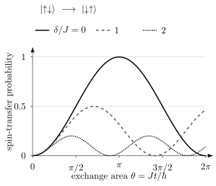
Exact constant-pulse probabilities in the antiparallel-spin subspace. Increasing $|\delta|/J$ raises the oscillation frequency but lowers the maximum transfer. Faster oscillations alone therefore do not imply a faster SWAP gate.

Why exchange is both useful and difficult

Exchange can be fast because it comes from wave-function overlap and virtual charge motion. It is usually controlled by barrier or detuning voltages, and often varies approximately exponentially over part of the operating range:

$$J(V) \approx J_0 e^{\alpha V}.$$

Then a small voltage fluctuation produces

$$\frac{\delta J}{J} \approx \alpha\,\delta V.$$

The same electrical leverage that makes a fast gate also amplifies charge noise and waveform distortion. A gate calibrated by exchange oscillations can still fail in a circuit because neighboring pulses, sensor states, or slow drift change the operating point.

Symmetric operation

For a double dot, let $\varepsilon$ denote detuning and $v_b$ a barrier coordinate. Near a charge-symmetric point,

$$\left. \frac{\partial J}{\partial\varepsilon} \right|_{\varepsilon=0} \approx0.$$

Detuning noise then enters at second order:

$$\delta J \approx \frac12 \frac{\partial^2J}{\partial\varepsilon^2} (\delta\varepsilon)^2 + \frac{\partial J}{\partial v_b}\delta v_b.$$

For zero-mean Gaussian detuning noise with variance $\sigma_\varepsilon^2$, the quadratic term also shifts the mean exchange by $J''\sigma_\varepsilon^2/2$. After recalibrating that shift, the fluctuation is $J''[(\delta\varepsilon)^2-\sigma_\varepsilon^2]/2$, with variance $(J'')^2\sigma_\varepsilon^4/2$. First-order insensitivity does not mean zero fluctuations. Symmetric-operation experiments by Reed and colleagues and Martins and colleagues illustrate the reduction of this noise pathway. Barrier noise, cross-capacitance, pulse distortion, nuclear gradients, and leakage remain. A “sweet spot” is always a derivative statement with respect to specified coordinates.

Long-range couplers

Direct exchange falls rapidly with distance. Proposed and demonstrated extensions include:

• physically shuttling electrons between interaction zones;
• superexchange through intermediate empty or occupied dots;
• capacitive coupling between charge-admixed spin encodings;
• coupling electric dipoles to superconducting microwave resonators;
• donor-register links through exchange-coupled electrons.

Each method changes the error channel. Shuttling risks transport leakage and phase pickup; superexchange introduces virtual-state sensitivity; capacitive and resonator couplings require charge or spin–photon admixture and can expose the spin to electric loss. Connectivity should be quoted with gate time, fidelity, concurrency, idle impact, and required intermediate hardware.

Noise and leakage

Residual nuclear spins

Natural silicon contains spinful $^{29}\mathrm{Si}$. Isotopic enrichment in $^{28}\mathrm{Si}$ can strongly reduce the fluctuating Overhauser field, but the residual concentration, spatial distribution, and nearby spinful materials still matter. Si/SiGe stacks may also contain spinful $^{73}\mathrm{Ge}$. Slow nuclear fluctuations often appear as qubit-frequency drift or quasi-static dephasing rather than a memoryless phase-flip channel.

Enrichment improves magnetic coherence but does not remove charge noise, valley disorder, control errors, or phonon-mediated relaxation. A long dynamically decoupled $T_2$ must not be used as a substitute for gate or code performance.

Charge noise

Charge fluctuators in oxides, interfaces, dielectrics, gates, and reservoirs shift dot potentials and tunnel barriers. They affect:

• exchange amplitudes and conditional phases;
• electric-dipole spin resonance through dot motion;
• Stark-shifted qubit frequencies and $g$ factors;
• valley and orbital energies;
• spin-to-charge conversion and sensor thresholds.

Low-frequency noise causes drift and nonexponential Ramsey decay. Noise near gate modulation frequencies causes stochastic gate error. Rare switching events can produce non-Gaussian tails. One spectral-density number cannot replace time-domain stability and contextual circuit tests.

Valley and orbital leakage

If a control pulse approaches an avoided crossing involving a valley or orbital state, nonadiabatic transitions can populate it. A simple Landau–Zener estimate for an isolated avoided crossing is

$$P_{\mathrm{LZ}} \approx \exp \left( -\frac{2\pi\Delta^2}{\hbar v} \right).$$

Here $2\Delta$ is the minimum gap and $v=|d(E_1-E_2)/dt|>0$ is the slope of the uncoupled energy difference. For an initial lower adiabatic eigenstate and a long linear sweep through the crossing, this is the probability of ending in the upper adiabatic branch (equivalently remaining on the initial diabatic branch). Whether that outcome constitutes leakage depends on which states encode the qubit. Real devices can have multiple crossings, dephasing, and pulse-dependent matrix elements, so the formula is a diagnostic scale rather than a complete leakage model.

Valley leakage can return coherently and masquerade as phase error, remain outside the code space, or alter a later measurement. Benchmarking that assumes a trace-preserving qubit channel can miss it.

Spin relaxation and hot spots

Spin–orbit and hyperfine admixture allow phonons or electrical noise to flip a spin. Near a spin–valley anticrossing, relaxation can be enhanced strongly. $T_1$ therefore depends on field, gate voltages, temperature, valley splitting, and device orientation. It must be measured near the actual operating points, including readout and shuttling configurations.

Leakage in encoded qubits

Singlet–triplet and exchange-only qubits use only part of a multi-spin Hilbert space. Transverse fields can enter polarized triplets; nonuniform fields or anisotropic exchange can mix total-spin sectors. Isotropic exchange alone preserves total spin, even with inaccurate pulse areas. Leakage can persist across many cycles and create correlated faults when a leaked spin interacts with neighbors.

A leakage-reduction unit may swap or reset leaked population through an ancilla or reservoir. Its cost includes extra exchange pulses, idle exposure, reset error, and schedule depth. Reporting a low in-subspace gate error while omitting leakage is incomplete.

Drift, context, and correlation

Qubit frequencies, exchange curves, tunnel rates, and sensor thresholds drift on different timescales. Feedback can keep one parameter locked while moving another. Shared controls and reservoirs can correlate errors spatially; low-frequency drift can correlate them temporally.

Fault-tolerance models need more than average gate infidelity. Useful diagnostics include leakage rates, simultaneous randomized benchmarking, cycle benchmarking, repeated-syndrome correlations, detector-event graphs, and held-out circuit prediction.

Temperature and Cryogenic Architecture

Thermal polarization and operating temperature

For an electron with $g^\ast\approx2$,

$$\frac{E_Z}{h} \approx 28\ \mathrm{GHz} \left( \frac{B}{1\ \mathrm T} \right),$$

while

$$\frac{k_BT}{h} \approx 20.8\ \mathrm{GHz} \left( \frac{T}{1\ \mathrm K} \right).$$

Operation above $1\ \mathrm K$ is possible when initialization and readout do not rely solely on thermal Zeeman polarization and when orbital, valley, charging, and reservoir scales remain suitable. Huang and colleagues demonstrate initialization and operation above $1\ \mathrm K$ in a two-qubit device. It does not show that a large processor, its amplifiers, its interconnects, and its fault-tolerant cycle all operate at that temperature.

Where the classical controller lives

Dense spin arrays create a wiring problem even though each qubit is small. Possible partitions include:

1. room-temperature waveform generation with filtered lines to the millikelvin stage;
2. cryogenic multiplexers or controllers at an intermediate stage near $1$–$4\ \mathrm K$;
3. selected digital or analog electronics at the millikelvin stage;
4. shared, crossbar, or globally broadcast controls with local selectivity.

Moving electronics colder reduces cable count and latency but consumes cooling power and can inject electrical or magnetic noise. Moving it warmer requires high-density low-thermal-conductance links with adequate bandwidth and signal integrity. A credible architecture states power per channel, static bias count, update rate, conversion resolution, line heat leak, sensor bandwidth, and feedback latency.

Cryogenic and Vacuum Infrastructure explains how heat flow, wiring, shielding, and amplifier noise constrain this division of the electronics.

Fabrication, Yield, and Automated Operation

Fabrication and few-electron uniformity

Silicon spin devices can use industrial materials, lithography, gate stacks, vias, and wafer-scale metrology. However, a transistor process optimized for classical threshold voltage, mobility, and leakage is not automatically optimized for few-electron disorder, valley splitting, charge noise, and coherent exchange.

Neyens and colleagues illustrate wafer-scale single-electron characterization. Fabrication and processor measurements answer different questions:

• geometric yield and dimensional variation;
• ability to accumulate and isolate single electrons;
• charge-noise and valley-splitting distributions;
• qubit coherence and gate performance across devices;
• simultaneous operation of a connected array;
• back-end routing, packaging, and cryogenic-controller integration.

Success at one level is valuable without proving the next.

Variability consumes control resources

Suppose device parameters $\theta_i$ have a distribution with mean $\bar\theta$ and spread $\sigma_\theta$. A controller can compensate some variation by per-qubit biases and pulse parameters, but each compensation consumes memory, calibration time, voltage range, and crosstalk margin. Fabrication uniformity and control sophistication are therefore interchangeable only within limits.

Yield also compounds. If a required unit cell succeeds independently with probability $y$, an unrepairable array of $N$ cells succeeds with probability

$$P_{\mathrm{array}} = y^N.$$

Independence is rarely exact, but the formula shows why spare cells, rerouting, defect maps, and repairable architectures matter even when $y$ is high.

Retuning reduces available experimental time

A processor with fast nanosecond exchange pulses can still have slow availability if loading, mapping charge transitions, fitting crosstalk, locking frequencies, and validating gates require extensive intervention. For disjoint categories of elapsed time, write

$$T_{\mathrm{scheduled}} = t_{\mathrm{experiment}} + t_{\mathrm{recalibration}} + t_{\mathrm{reload}} + t_{\mathrm{recovery}}.$$

The relevant fraction is useful experimental time divided by total scheduled time, with failures and retuning included.

Processor Metrics

The generic definitions in Metrics for Quantum Hardware apply, but silicon spin processors need several additional labels.

Quantity	Ambiguity to remove
dot count	Does every dot contain a controlled spin? Are some dots buses, sensors, reservoirs, or leakage sinks?
physical-spin count	Are electrons, nuclei, readout ancillas, and mobile ancillas all included?
encoded-qubit count	Does one qubit consume one, two, or three spins?
connected count	Which pairs have calibrated entangling operations in the same configuration?
active count	Which qubits are initialized, controlled, and measured in one experiment?
logical count	Is the code detecting or correcting errors, and are logical gates protected?

For an exchange gate, report pulse duration, exchange area, leakage, single-qubit phase corrections, spectator conditions, and benchmark protocol. For readout, report spin-to-charge conversion, sensor assignment, integration time, relaxation correction, and whether assignment is simultaneous. For shuttling, report distance, time, number of segments, state fidelity, phase calibration, charge-survival probability, and the extrapolation model.

For a fully serial schedule with disjoint stages, a cycle time is

$$t_{\mathrm{cycle}} = t_{\mathrm{entangle}} + t_{\mathrm{ancilla\ measure}} + t_{\mathrm{reset}} + t_{\mathrm{feedback}} + t_{\mathrm{routing}} + t_{\mathrm{idle}}.$$

Fast exchange alone may be a small part of this sum. With pipelining or parallel operations, elapsed time follows the schedule’s critical path. An idle error can accrue while another qubit is measured, so that exposure must not be counted again as an extra elapsed-time stage.

Error detection and correction

Component thresholds are conditional

A physical gate fidelity above a quoted surface-code threshold is encouraging only after matching the assumed noise model, leakage treatment, connectivity, measurement schedule, and simultaneous-operation conditions. There is no platform-independent rule that “above $99\%$” means fault tolerant.

The stronger experiment repeats syndrome extraction, decodes the record, and tests whether logical error falls when code distance or another protection resource increases under comparable conditions.

Error detection is not error correction

The $[[4,2,2]]$ code encodes two logical qubits and detects any single-qubit Pauli error, but distance two cannot identify and correct an arbitrary single-qubit error without additional information. One known-location erasure is correctable in principle; an unknown-location arbitrary error is not. Postselecting on a clean syndrome can raise conditional fidelity while lowering throughput:

$$R_{\mathrm{accepted}} = R_{\mathrm{shots}}\, p_{\mathrm{accept}}.$$

Both quantities must be reported. A universal set of operations on encoded states is a major control result, but it does not by itself demonstrate that logical error decreases with code distance or that operations are fault-tolerant under repeated correction.

A weight-four stabilizer measurement tests a useful interaction-and-readout primitive. A repeated quantum memory must additionally protect against both bit and phase errors, control leakage, decode imperfect measurements, and show the expected scaling. A repetition code still has a two-dimensional logical space and can protect an arbitrary superposition against one specified Pauli error type; its orthogonal error type remains unprotected. See Why Quantum Error Correction Is Possible and Surface Code for those distinctions.

Exercises

1. Thermal polarization

Take an electron with $g^\ast=2$ at $B=1\ \mathrm T$. Estimate its ground-state thermal population at $T=100\ \mathrm{mK}$ and $T=1\ \mathrm K$. Use $\mu_B=57.9\ \mu\mathrm{eV/T}$ and $k_B=86.2\ \mu\mathrm{eV/K}$. Explain why a hot-qubit experiment may require algorithmic initialization.

Solution

The Zeeman splitting is

$$E_Z = g^\ast\mu_BB \approx 115.8\ \mu\mathrm{eV}.$$

At $100\ \mathrm{mK}$,

$$\frac{E_Z}{k_BT} \approx \frac{115.8}{8.62} \approx 13.4,$$

so

$$p_g = \frac{1}{1+e^{-13.4}} \approx 0.9999985.$$

At $1\ \mathrm K$,

$$\frac{E_Z}{k_BT} \approx \frac{115.8}{86.2} \approx 1.34,$$

and

$$p_g \approx \frac{1}{1+e^{-1.34}} \approx 0.79.$$

Thermal waiting at $1\ \mathrm K$ therefore leaves roughly one spin in five excited in this ideal two-level estimate. Measurement, feedback, entropy transfer, or energy-selective loading is needed for high-purity initialization.

2. Exchange pulse area

Two spins have a constant exchange frequency $J/h=20\ \mathrm{MHz}$. Neglect all Zeeman gradients and pulse ramps. Find the duration of a $\sqrt{\mathrm{SWAP}}$ pulse.

Solution

The exchange area is

$$\theta = \frac{J\tau}{\hbar} = 2\pi \frac{J}{h}\tau.$$

For $\sqrt{\mathrm{SWAP}}$, $\theta=\pi/2$, so

$$\tau = \frac{1}{4(J/h)} = \frac{1}{80\ \mathrm{MHz}} = 12.5\ \mathrm{ns}.$$

A real pulse needs ramp corrections, single-qubit phase tracking, and a leakage check.

3. Charge-noise leverage

Assume $J(V)=J_0e^{\alpha V}$ with $\alpha=20\ \mathrm{V}^{-1}$. Estimate the fractional exchange error caused by a quasi-static voltage offset of $10\ \mu\mathrm V$. What phase error does this produce for an otherwise ideal $\sqrt{\mathrm{SWAP}}$ pulse?

Solution

To first order,

$$\frac{\delta J}{J} \approx \alpha\delta V = 20\times10^{-5} = 2\times10^{-4}.$$

For fixed duration, the exchange area has the same fractional error:

$$\delta\theta \approx \frac{\pi}{2} \left(2\times10^{-4}\right) \approx 3.1\times10^{-4}\ \mathrm{rad}.$$

This is only the quasi-static contribution from the chosen voltage coordinate. Broadband noise and pulse distortion require a filter-function or full control model.

4. A two-dot virtual gate

Near one operating point, suppose

$$\begin{pmatrix} \delta\mu_1\\ \delta\mu_2 \end{pmatrix} = \begin{pmatrix} 1&0.2\\ 0.1&1 \end{pmatrix} \begin{pmatrix} \delta V_1\\ \delta V_2 \end{pmatrix}.$$

Find physical voltage changes that shift only dot 1 by $\delta$.

Solution

The determinant is $1-0.02=0.98$. Inverting the matrix gives

$$\begin{pmatrix} \delta V_1\\ \delta V_2 \end{pmatrix} = \frac{1}{0.98} \begin{pmatrix} 1&-0.2\\ -0.1&1 \end{pmatrix} \begin{pmatrix} \delta\\ 0 \end{pmatrix}.$$

Therefore

$$\delta V_1 = \frac{\delta}{0.98}, \qquad \delta V_2 = -\frac{0.1\delta}{0.98}.$$

The compensating change on gate 2 cancels its first-order influence on $\mu_2$. The calibration remains local and must be updated if the cross-capacitance matrix changes.

5. Coherent and independent transport errors

Each of two transport segments introduces $U=\exp(-i\phi Z/2)$ with $\phi=0.02$. For an input $\lvert+\rangle$, compare the two-segment return probability with the square of the one-segment probability. What changes if the second segment introduces $U^\dagger$?

Solution

One segment gives $F_1=\cos^2(\phi/2)\approx0.9999000033$. Two identical coherent errors give $F_2=\cos^2\phi\approx0.9996000533$, whereas $F_1^2\approx0.9998000167$. The infidelity grows quadratically with the accumulated angle, not as the sum of independent failure probabilities. With the opposite second rotation, $U^\dagger U=I$ and $F_2=1$. Calibration that reveals only one input-state fidelity cannot determine how an error composes along a route.

6. Readout is a response matrix

Let $F_\downarrow=0.99$ be the probability of declaring down when the spin is down, and $F_\uparrow=0.97$ the probability of declaring up when it is up. For an equal prior mixture, find the probability of an up declaration and the posterior probability that the spin was actually up given that declaration.

Solution

The up-declaration probability is

$$\begin{aligned} P(d_\uparrow) &= \frac12(1-F_\downarrow) + \frac12F_\uparrow \\ &= \frac12(0.01+0.97) = 0.49. \end{aligned}$$

Bayes’ rule gives

$$\begin{aligned} P(\uparrow\mid d_\uparrow) &= \frac{ P(d_\uparrow\mid\uparrow)P(\uparrow) }{ P(d_\uparrow) } \\ &= \frac{0.97\times0.5}{0.49} \approx 0.990. \end{aligned}$$

Assignment fidelity and posterior confidence depend on different conditionals; the latter also depends on the input prior.

7. Yield compounding

An unrepairable design needs 1,000 statistically independent unit cells. If each has yield $y=0.999$, what is the complete-array yield? What architecture lesson follows?

Solution

The idealized array yield is

$$P_{\mathrm{array}} = 0.999^{1000} \approx e^{-1} \approx 0.368.$$

A seemingly high cell yield leaves only about $37\%$ perfect arrays at this size. Larger systems need better yield, spare cells, defect-aware mapping, repair, or routing around failures. Correlated wafer defects can make the independent model optimistic or pessimistic, so measured spatial statistics are required.

8. Postselected error detection

A $[[4,2,2]]$ experiment prepares encoded states, runs logical gates, rejects shots with nontrivial syndromes, and reports higher fidelity on accepted shots. What has been demonstrated, and what two quantities are required to interpret the result?

Solution

The experiment demonstrates encoded state preparation, logical control, and single-error detection in the tested circuits. It may also demonstrate fault-tolerant construction of selected operations under explicit fault-propagation criteria.

It does not demonstrate arbitrary single-error correction or distance scaling because the code has distance two. At minimum one must report both the conditional logical fidelity and the acceptance probability or accepted throughput. Otherwise postselection can make the retained sample look better while discarding most attempts.

9. Exchange in a field gradient

Take $J/h=20\ \mathrm{MHz}$ and $\delta=J$. Find the time and probability of the first transfer maximum. Compare it with the zero-gradient SWAP time.

Solution

The first maximum obeys $\sqrt2 Jt/(2\hbar)=\pi/2$, giving $t=h/(2\sqrt2 J)\approx17.68\ \mathrm{ns}$ and $P=1/2$. At zero gradient, the first maximum is at $t=h/(2J)=25\ \mathrm{ns}$ and reaches unity. The earlier maximum at nonzero gradient is incomplete transfer, so it is not a faster implementation of SWAP.

References

• G. Burkard, T. D. Ladd, A. Pan, J. M. Nichol, and J. R. Petta, “Semiconductor spin qubits,” Reviews of Modern Physics 95, 025003 (2023), doi:10.1103/RevModPhys.95.025003.

• J. M. Elzerman et al., “Single-shot read-out of an individual electron spin in a quantum dot,” Nature 430, 431–435 (2004), doi:10.1038/nature02693.

• R. Hanson, L. P. Kouwenhoven, J. R. Petta, S. Tarucha, and L. M. K. Vandersypen, “Spins in few-electron quantum dots,” Reviews of Modern Physics 79, 1217–1265 (2007), doi:10.1103/RevModPhys.79.1217.

• J. Y. Huang et al., “High-fidelity spin qubit operation and algorithmic initialization above $1\ \mathrm K$,” Nature 627, 772–777 (2024), doi:10.1038/s41586-024-07160-2.

• B. E. Kane, “A silicon-based nuclear spin quantum computer,” Nature 393, 133–137 (1998), doi:10.1038/30156.

• D. Loss and D. P. DiVincenzo, “Quantum computation with quantum dots,” Physical Review A 57, 120–126 (1998), doi:10.1103/PhysRevA.57.120.

• F. Martins, F. K. Malinowski, P. D. Nissen, E. Barnes, S. Fallahi, G. C. Gardner, M. J. Manfra, C. M. Marcus, and F. Kuemmeth, “Noise suppression using symmetric exchange gates in spin qubits,” Physical Review Letters 116, 116801 (2016), doi:10.1103/PhysRevLett.116.116801.

• A. Morello et al., “Single-shot readout of an electron spin in silicon,” Nature 467, 687–691 (2010), doi:10.1038/nature09392.

• S. Neyens et al., “Probing single electrons across 300-mm spin qubit wafers,” Nature 629, 80–85 (2024), doi:10.1038/s41586-024-07275-6.

• J. J. Pla et al., “A single-atom electron spin qubit in silicon,” Nature 489, 541–545 (2012), doi:10.1038/nature11449.

• M. D. Reed et al., “Reduced sensitivity to charge noise in semiconductor spin qubits via symmetric operation,” Physical Review Letters 116, 110402 (2016), doi:10.1103/PhysRevLett.116.110402.

• P. Stano and D. Loss, “Review of performance metrics of spin qubits in gated semiconducting nanostructures,” Nature Reviews Physics 4, 672–688 (2022), doi:10.1038/s42254-022-00484-w.

• M. Veldhorst et al., “A two-qubit logic gate in silicon,” Nature 526, 410–414 (2015), doi:10.1038/nature15263.

• A. J. Weinstein et al., “Universal logic with encoded spin qubits in silicon,” Nature 615, 817–822 (2023), doi:10.1038/s41586-023-05777-3.

• F. A. Zwanenburg et al., “Silicon quantum electronics,” Reviews of Modern Physics 85, 961–1019 (2013), doi:10.1103/RevModPhys.85.961.