Materials and Fabrication Interface

Materials influence quantum hardware through two distinct effects: they set the noise and loss experienced by each device, and they create variation between devices. A low-loss material can still produce poorly matched resonances; a uniform process can still make uniformly noisy qubits. Geometry, packaging, and calibration determine how these properties affect useful operations.

This page connects material properties and fabrication distributions to quantum-device performance, screening, yield, and reliability. For contacts, patterning, and assembly, see Device Fabrication Concepts. For the resulting thermal and vacuum environment, see Cryogenic and Vacuum Infrastructure.

Required background. Hardware Overview defines the physical components of a quantum device; Metrics for Quantum Hardware distinguishes coherence and operation errors; Control, Readout, and Calibration explains how device parameters are estimated and adjusted.

Material variation and device sensitivity

Let $\mathbf x$ contain material properties, geometry, assembly conditions, and environment, and let $\mathbf u$ contain tunable controls. A measured device vector has the form

$$\mathbf z=\mathcal F(\mathbf x,\mathbf u)+\boldsymbol\epsilon.$$

Examples of $\mathbf z$ are transition frequencies, decay rates, tunnel couplings, and optical linewidths. The measurement protocol is fixed when comparing this map across devices. Static offsets, temporal fluctuations, and measurement error must remain distinct: a frequency offset may be calibrated away, whereas fluctuations during an operation cause dephasing.

At fixed control settings, small variations around a smooth operating point give

$$\delta\mathbf z\simeq J\delta\mathbf x+\boldsymbol\epsilon, \qquad J_{\alpha i}=\frac{\partial z_\alpha}{\partial x_i}.$$

For zero-mean measurement error uncorrelated with $\delta\mathbf x$,

$$\Sigma_z\simeq J\Sigma_xJ^{\mathsf T}+\Sigma_\epsilon.$$

Otherwise cross-covariance terms are also present. This linear approximation can fail near a charge transition, crack, defect-charge switching event, or other discontinuity. It also misses curvature-induced mean shifts when variations are not small.

Correlations can help one observable and harm another. For equal frequency standard deviations $\sigma$ and correlation coefficient $\rho$,

$$\operatorname{Var}(f_1-f_2)=2\sigma^2(1-\rho).$$

A shared process shift can cancel in a detuning while moving both frequencies outside a fixed control band. Separate one-dimensional histograms do not contain this information.

Noise strength and susceptibility

For real, stationary classical fluctuations, define the two-sided angular- frequency cross spectrum by

$$S_{ij}(\Omega)=\int_{-\infty}^{\infty} e^{i\Omega\tau}\, \langle\delta x_i(t+\tau)\delta x_j(t)\rangle\,d\tau.$$

If $\delta\omega(t)\simeq\sum_i g_i\delta x_i(t)$, with real $g_i=\partial\omega/\partial x_i$, then

$$S_\omega(\Omega)=\sum_{ij}g_iS_{ij}(\Omega)g_j.$$

Reducing a noise source and reducing its coupling to the device are different interventions. A sweet spot suppresses a first derivative without removing the fluctuators. Quadratic sensitivity, transverse noise, and drift can remain. Quantum bath spectra and protocol-dependent dephasing require the conventions in Noise Spectra and One-Over-F Noise.

Example: junction resistance and transmon frequency

In the large-$E_J/E_C$ transmon approximation (Koch and colleagues),

$$hf_{01}\simeq\sqrt{8E_JE_C}-E_C.$$

For equivalent tunnel junctions at fixed gap and temperature, the Ambegaokar–Baratoff relation makes $I_cR_n$ approximately constant, so $E_J=\hbar I_c/(2e)\propto R_n^{-1}$. Here $R_n$ is the normal-state resistance of the junction. An accessible room-temperature measurement is a proxy whose relation to this parameter must itself be checked.

Keeping $E_C$ fixed and differentiating gives

$$\frac{\delta f_{01}}{f_{01}} \simeq-\frac12\left(1+\frac{E_C}{hf_{01}}\right) \frac{\delta R_n}{R_n}.$$

Thus the often-used half-as-large fractional spread additionally neglects $E_C/(hf_{01})$. For $f_{01}=5\,\mathrm{GHz}$ and $E_C/h=0.25\,\mathrm{GHz}$, a small $2\%$ resistance spread gives about $1.05\%$ frequency spread. Changing capacitance or superconducting gap adds other derivatives and correlations. This model predicts frequency targeting, not coherence or simultaneous gate performance. Van Damme and colleagues provide a fabrication example of resistance and frequency distributions.

Participation and material loss

A material matters most where the mode stores energy. For a weakly lossy, approximately nondispersive dielectric and a nearly harmonic mode, define the fraction of electric-field energy in region $i$ by

$$p_i= \frac{\int_{V_i}\epsilon_i'|\mathbf E|^2\,dV} {\int_{\mathrm{all}}\epsilon'|\mathbf E|^2\,dV}.$$

The ratio uses electric energy in both numerator and denominator. At resonance, equal time-averaged electric and magnetic energies lead to

$$\begin{aligned} Q_{\mathrm{int}}^{-1}&\simeq\sum_i p_i\tan\delta_i+Q_{\mathrm{other}}^{-1},\\ \Gamma_{1,\mathrm{diel}}&\simeq\omega\sum_i p_i\tan\delta_i. \end{aligned}$$

$Q=\omega U/P_{\mathrm{loss}}$ describes energy decay, and $T_1=Q/\omega$ when that decay is exponential. The model also approximates dielectric loss of a weakly anharmonic qubit. Strong coupling to an individual defect, frequency-dependent hybridization, or nonexponential decay requires a more specific dynamical model.

The effective loss tangent can depend on temperature, frequency, field orientation, processing, and excitation power. Saturating two-level defects with a strong drive can make a resonator appear less lossy than in the single-photon regime. Interface thickness and permittivity also enter the calculated participation. Martinis and colleagues, Wang and colleagues, and Ganjam and colleagues establish complementary microscopic, geometrical, and multimode approaches to this problem.

Separating losses with several modes or geometries

After subtracting independently established background losses, suppose measurements satisfy

$$\mathbf q=P\boldsymbol d+\boldsymbol\eta, \qquad q_k=Q_k^{-1},\quad d_i=\tan\delta_i.$$

Every row of $P$ gives one mode’s participations. Unknown background losses need additional parameters; they cannot simply be subtracted as if known. The modes must sample the same loss factors for this combined model to apply.

If $P$ has full column rank, noiseless data determine $\boldsymbol d$. Proportional columns leave an exact ambiguity. Nearly proportional columns instead give a unique but noise-sensitive estimate. For known $P$ and independent measurement noise of variance $\sigma_q^2$, least squares gives

$$\operatorname{Cov}(\widehat{\boldsymbol d}) =\sigma_q^2(P^{\mathsf T}P)^{-1}.$$

Repeating the same independent measurements $m$ times reduces this covariance by $1/m$, while leaving the condition number unchanged. It cannot remove an exact null space. Changing the relative participations can improve sensitivity to the previously weakly constrained loss combination. Systematic field-model errors and actual device-to-device loss variation do not average away like independent instrument noise.

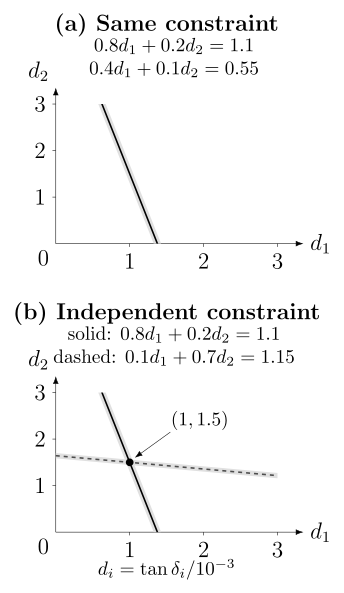
(a) The two equations constrain the same combination of loss tangents. (b) A different participation vector supplies a second direction and locates the intersection at $(d_1,d_2)=(1,1.5)$. Here the plotted variables are loss tangents in units of $10^{-3}$; shaded bands illustrate finite measurement uncertainty, rather than a statistical confidence region for the joint fit.

Ganjam and colleagues used multiple resonator modes to distinguish surface, bulk, and package losses and then tested predictions for other devices. The transferable idea is to change sensitivity deliberately, rather than attribute every improvement to the material named in the fabrication change.

Physical changes introduced by fabrication

The relevant material state includes composition, isotope, defects, strain, interfaces, and processing history. Several recurring mechanisms explain why these details survive into the quantum experiment.

Isotopes and impurities. Reducing spinful nuclei suppresses one magnetic bath, as illustrated by Tyryshkin and colleagues in silicon and Balasubramanian and colleagues in diamond. It does not remove charge traps, paramagnetic contamination, or control noise. A desired donor or color center must also have the appropriate position, charge state, and environment.

Surfaces and interfaces. Metal edges, semiconductor–oxide boundaries, waveguide sidewalls, and shallow defects can concentrate fields or wavefunctions near noisy regions. An effective two-level fluctuator is a model, not a unique chemical identification. Microscopy of one sharp interface does not establish its noise spectrum or spatial uniformity. Hite and colleagues’ controlled ion-trap cleaning experiment demonstrates a surface contribution to heating without identifying a universal mechanism for every trap.

Dimensions and strain. Junction area, barrier thickness, gate gaps, waveguide cross-sections, and implantation positions change energies and couplings. Nominal layout, measured geometry, and effective electrical or optical dimensions need not coincide. Cooldown strain can shift defect transitions and valley splittings even when room-temperature dimensions pass inspection.

Assembly. Bonding, seams, interposers, fiber alignment, and enclosure modes can alter a screened die. Compare the same devices before and after packaging and cooldown to separate this change from selection of a different sample.

Device	Material or process effect	Useful comparison
Superconducting circuit	Interface loss and junction dispersion	Low-power loss across several participations; resistance versus measured frequency
Silicon spin array	Charge disorder, valley splitting, gate variation	One-electron tuning and simultaneous control, beyond gate continuity
Solid-state emitter	Placement, charge state, strain, surface noise	Track the same emitters through fabrication and optical integration
Photonic circuit	Propagation loss, coupler imbalance, phase offsets	Low-power transmission and interference before and after packaging
Trapped ion	Surface electric-field noise	Heating versus controlled surface treatment, distance, and temperature
Hybrid semiconductor–superconductor	Interface transparency and subgap states	Structural characterization together with gap spectroscopy

Neyens and colleagues demonstrate why electrical dot yield and shared-voltage compatibility are different quantities. Sutula and colleagues demonstrate automated optical tracking and screening of emitters; screening finds useful devices but does not create identical emitters deterministically. A hard induced gap, as in Chang and colleagues’ experiment, is a useful interface result but does not alone establish a topological phase or protected qubit. Detailed encodings and operations are developed in the linked hardware platform pages.

Screening and usable yield

A test structure deliberately emphasizes one mechanism while being easier to measure than the final device: a resonator, junction array, Hall bar, waveguide, or witness surface. Its usefulness depends on predicting the quantity of interest under the intended conditions. Mobility alone does not predict the noise of one gate-defined dot; a bright emitter is not necessarily an indistinguishable single-photon source.

Check predictions on devices or batches excluded from fitting. A changed geometry, package, material source, or temperature can change the relation between the proxy and its target.

A screening pass is conditional information

Let $S$ denote passing an early screen and $U$ final usability. Then

$$\begin{aligned} \text{sensitivity}&=P(S\mid U),\\ \text{specificity}&=P(\neg S\mid\neg U),\\ \text{precision}&=P(U\mid S). \end{aligned}$$

The last quantity depends on the prevalence $P(U)$, not only on sensitivity and specificity. Hand-selected good and bad examples need not reproduce that prevalence. False rejects discard useful devices; false passes consume later packaging, cooling, and calibration time. Guard bands account for measurement uncertainty near specification limits; JCGM 106 treats the associated conformance-decision risks.

Component yield is not system yield

For a joint acceptance region $\mathcal A$ in device-parameter space,

$$Y_{\mathrm{dev}}=P(\mathbf z\in\mathcal A).$$

Marginal pass rates for separate metrics do not determine this probability. Moreover, passing tests in isolation does not establish simultaneous operation in the presence of crosstalk and shared controls.

If all $N$ components are required and independent, each with usable probability $y$, then $Y_{\mathrm{all}}=y^N$. Thus $0.99^{1000}\simeq4.3\times10^{-5}$. This motivates higher yield, spares, repair, or architectures that tolerate some defects; it is not a universal prediction for a processor.

Let $E_{\mathrm{graph}}$ mean that working components form the required connected arrangement, and $E_{\mathrm{joint}}$ that they operate together within the relevant limits. The actual quantity is

$$Y_{\mathrm{sys}}=P(E_{\mathrm{graph}}\cap E_{\mathrm{joint}}).$$

Correlations have no universal sign of effect on this probability. Perfectly correlated failures can increase the chance that all components are good at a fixed marginal yield, while making the failing cases more catastrophic. Exercise 4 gives an explicit example. Spatial placement matters when only certain patterns can be bypassed.

Always identify the sampled population. Gate continuity, one-electron dots, calibrated qubits, and simultaneously operable arrays have different denominators. A coherence histogram restricted to working devices answers a conditional question and does not estimate unconditional fabrication yield.

Sampling uncertainty and process comparisons

Many devices from one wafer do not constitute many independent tests of a wafer-level process change. A simple hierarchical model separates lot, wafer, die, device, and cooldown contributions:

$$z_{\ell w d i c} =\mu+a_\ell+b_{\ell w}+c_{\ell wd} +u_{\ell wdi}+v_{\ell wdic}+\epsilon.$$

The terms describe scales of variation, not proven microscopic mechanisms. Repeated spectra estimate measurement or time variation; they do not add independent wafers. A common cooldown shared by several devices also calls for a shared cooldown term rather than independent device-specific offsets.

Estimating a pass probability

Suppose pass/fail outcomes are independent conditional on one common probability $y$, so $k\mid y\sim\operatorname{Binomial}(n,y)$. With a uniform prior,

$$y\mid k,n\sim\operatorname{Beta}(k+1,n-k+1).$$

The posterior mean is $(k+1)/(n+2)$. Exchangeability by itself does not justify this binomial likelihood: finite-population sampling, spatially clustered failures, or batch-dependent probabilities require their own models. Frequentist binomial confidence intervals likewise depend on a sampling model. Neither approach makes five successes a precise estimate of near-perfect yield.

Uncertainty in $y$ also matters when predicting a future assembly. Under the same conditional-independence model, average $y^N$ over its posterior:

$$P(\text{all }N\text{ pass}\mid k,n) =\mathbb E[y^N\mid k,n].$$

This is generally not $(\mathbb E[y\mid k,n])^N$. The predictive dependence from an uncertain shared parameter is distinct from a physical common-cause failure. Exercise 12 calculates the difference.

Process capability and causal inference

For a stable, approximately normal scalar process, the common capability index is

$$C_{pk}=\min\left[ \frac{\mathrm{USL}-\mu}{3\sigma}, \frac{\mu-\mathrm{LSL}}{3\sigma}\right].$$

Its interpretation as a tail-risk summary requires the distributional and stability assumptions; the numerical ratio alone does not establish them. It also says nothing about whether that specification predicts a quantum metric. NIST’s statistical handbook discusses these limitations.

To test a surface treatment, compare matched or randomized specimens, block by wafer position and measurement session, and replicate at the level where the treatment is applied. If the treatment must be applied to an entire wafer, individual dies cannot serve as independent treatment assignments. Hold geometry and packaging fixed when testing chemistry; deliberately vary geometry when testing a participation model. A later batch and a geometry excluded from fitting provide stronger predictive checks than repeated measurements of the best device.

Tuning and reliability after fabrication

Tuning can compensate static offsets but consumes range, resolution, power, calibration time, and sometimes coherence. Near a smooth operating point, if calibration applies $\delta\mathbf u=K\delta\mathbf x$, the residual sensitivity is

$$\delta\mathbf z\simeq(J_x+J_uK)\delta\mathbf x.$$

Finite control range can prevent this cancellation; uncertainty in the estimated offset and actuator noise add residual error. Compare initial spread, corrected spread, and drift separately. Spectral tuning that removes a collision can move a qubit away from a noise sweet spot.

Yield describes acceptance at a given time. For the first failure of an accepted device, a nonnegative hazard $\lambda(t)$ gives survival

$$R(t)=\exp\left[-\int_0^t\lambda(t')\,dt'\right].$$

This is not the availability of a repairable device that can fail and return to service. Oxidation, adsorption, trapped charge, thermal cycling, package strain, and dose-dependent damage can produce nonconstant hazards. State whether the independent variable is calendar time, cold time, or cycle count. Units still working when observations end are right-censored; they retain information about survival. Modular Architectures develops the role of replacement and shared failures in a connected machine.

Exercises

1. Participation-limited lifetime

A $5\,\mathrm{GHz}$ mode has two dielectric contributions:

$$\begin{array}{c|cc} i & p_i & \tan\delta_i\\ \hline 1 & 2.0\times10^{-3} & 2.0\times10^{-3}\\ 2 & 4.0\times10^{-4} & 5.0\times10^{-4} \end{array}$$

Neglect other loss. Estimate $T_1$. Then halve $p_1$ without changing the frequency or loss tangents. By what factor does $T_1$ improve?

Solution

The total inverse quality factor is

$$\begin{aligned} Q^{-1} &= \sum_i p_i\tan\delta_i \\ &= 4.0\times10^{-6} + 2.0\times10^{-7} \\ &= 4.2\times10^{-6}. \end{aligned}$$

Using $T_1=Q/\omega$ with $\omega=2\pi(5\times10^9)\,\mathrm{s^{-1}}$,

$$\begin{aligned} T_1 &= \frac{1} {2\pi(5\times10^9)(4.2\times10^{-6})} \\ &\approx 7.6\,\mu\mathrm s. \end{aligned}$$

After halving $p_1$,

$$\begin{aligned} Q_{\mathrm{new}}^{-1} &= 2.0\times10^{-6} + 2.0\times10^{-7} \\ &= 2.2\times10^{-6}. \end{aligned}$$

So

$$T_{1,\mathrm{new}} \approx 14.5\,\mu\mathrm s.$$

The improvement is $4.2/2.2\approx1.91$, not exactly two, because the second loss channel remains.

2. Correlated fabrication shifts

Two resonances have fluctuations $\delta f_1$ and $\delta f_2$, each with standard deviation $10\,\mathrm{MHz}$ and correlation coefficient $0.8$. Find the standard deviation of their detuning $\Delta=f_1-f_2$. Compare with independent fluctuations.

Solution

For equal standard deviations $\sigma$,

$$\begin{aligned} \operatorname{Var}(\Delta) &= \operatorname{Var}(f_1) + \operatorname{Var}(f_2) -2\operatorname{Cov}(f_1,f_2)\\ &= 2\sigma^2(1-\rho). \end{aligned}$$

With $\sigma=10\,\mathrm{MHz}$ and $\rho=0.8$,

$$\sigma_\Delta = 10\sqrt{0.4}\,\mathrm{MHz} \approx 6.3\,\mathrm{MHz}.$$

For independent shifts, $\rho=0$ and $\sigma_\Delta=10\sqrt2\,\mathrm{MHz}\approx14.1\,\mathrm{MHz}$. A common process shift can broaden absolute frequencies while partly canceling in a local detuning. The same correlation could be harmful for a different architecture metric.

3. Scaling an all-required assembly

An architecture needs all $N=1000$ components and assumes independent usable probability $y=0.999$ per component.

1. Estimate the all-good yield.
2. Explain why a measured $99.9\%$ component yield is still insufficient to predict a real processor yield.

Solution

The simple estimate is

$$Y_{\mathrm{all}} = 0.999^{1000} \approx e^{-1.0005} \approx 0.368.$$

The approximation uses $\ln(0.999)\approx-0.0010005$. The real system may have spatially correlated failures, several component types, parameter-window failures, package defects, repair, spares, routing around faults, and graph constraints. The component number and the architecture’s acceptance rule are both needed.

4. Clustered failures

One hundred devices are arranged in ten process blocks of ten. In a simplified model, each complete block is good with probability $0.98$ and bad otherwise, independently between blocks. Every device therefore has marginal good probability $0.98$.

1. Find the probability that all 100 devices are good.
2. Compare with 100 independent devices of yield $0.98$.
3. What does the comparison teach?

Solution

All devices are good only when all ten blocks are good:

$$Y_{\mathrm{block}} = 0.98^{10} \approx 0.817.$$

Under independent device failures,

$$Y_{\mathrm{ind}} = 0.98^{100} \approx 0.133.$$

Positive within-block correlation increases the probability of a completely good assembly here, but failures occur in ten-device clusters. An architecture that tolerates a few isolated failures may fare much worse under the clustered model. Marginal component yield does not determine system yield; the failure geometry and acceptance rule do.

5. Uncertainty behind a yield claim

Nineteen of twenty independently sampled devices pass a fixed test. Using a uniform prior for pass probability $y$:

1. write the posterior distribution;
2. find its mean;
3. explain why neither $19/20$ nor the posterior mean should be advertised without an interval and sampling context.

Solution

The posterior is

$$y\mid k=19,n=20 \sim \operatorname{Beta}(20,2).$$

Its mean is

$$\mathbb E[y\mid k,n] = \frac{k+1}{n+2} = \frac{20}{22} \approx 0.909.$$

The raw fraction is $0.95$, but twenty observations leave substantial uncertainty about the underlying probability. The inference also assumes units sampled from the intended process and independent conditional on a common pass probability. Twenty devices from one selected die do not establish lot-level yield.

6. Process capability

A stable scalar process has mean $\mu=100$, standard deviation $\sigma=2$, lower specification limit $92$, and upper specification limit $106$. Compute $C_{pk}$ and identify the limiting side.

Solution

The two one-sided values are

$$\begin{aligned} \frac{\mathrm{USL}-\mu}{3\sigma} &= \frac{106-100}{6} =1, \\ \frac{\mu-\mathrm{LSL}}{3\sigma} &= \frac{100-92}{6} =\frac{4}{3}. \end{aligned}$$

Thus $C_{pk}=1$, limited by the upper specification. The calculation does not show that the process is stable, normal, uncorrelated, or predictive of a quantum metric; those assumptions require separate evidence.

7. Screening precision

A cryogenic screen has sensitivity $0.90$ and specificity $0.80$ for final device usability. Only $20\%$ of incoming devices are actually usable. Find the probability that a screened-pass device is usable.

Solution

Let $a=P(S\mid U)P(U)$ and $b=P(S\mid\neg U)P(\neg U)$ be the usable and unusable contributions. Bayes’ rule gives

$$\begin{aligned} a &= 0.90(0.20) =0.18, \\ b &= 0.20(0.80) =0.16, \\ P(U\mid S) &= \frac{a}{a+b} \approx0.529. \end{aligned}$$

Despite apparently respectable sensitivity and specificity, only about $53\%$ of passing devices are usable because the base rate is low. Screening thresholds must be evaluated on production prevalence and decision costs.

8. Identifiability in a loss experiment

Two test resonators have participation vectors

$$\mathbf p_1=(0.8,0.2), \qquad \mathbf p_2=(0.4,0.1)$$

for two unknown interface losses. Can their measurements determine both loss tangents? Propose a useful third participation vector.

Solution

No. The second vector is exactly one half of the first, so the participation matrix has rank one. Both measurements constrain the same weighted sum $0.8\delta_1+0.2\delta_2$.

A useful third design must not be proportional, for example

$$\mathbf p_3=(0.1,0.7).$$

The expanded matrix has rank two. With known other losses, noiseless data then determine both unknowns. Nearly proportional rows instead give a unique but noise-sensitive estimate. Independent repetitions reduce statistical uncertainty; changing the relative participations improves the conditioning. Neither repeated measurements nor positivity alone generally determine a unique solution to the original rank-one problem.

9. Design a split-lot experiment

A team believes a new surface clean lowers superconducting-device loss. Design a comparison that can distinguish the clean from wafer location, geometry, package, cooldown, and measurement-session effects.

Solution

Use at least several independent wafers or lots. Within each, randomize matched dies or resonator geometries between the old and new clean, while blocking by wafer region. Keep downstream geometry and package fixed, or balance package variants across both treatments. Measure witness surfaces and several participation geometries, then interleave device measurements within the same sessions and cryogenic environment.

Predeclare the primary loss metric, exclusions, and hierarchy-aware analysis. After model development, repeat the comparison on a held-out batch and test whether inferred loss factors predict a geometry not used in the fit. The independent replication count is the number of independently treated process units, not the number of repeated spectra.

10. What a hard gap establishes

A report states: “An epitaxial interface produced a hard induced gap, proving that the process yields protected topological qubits.” Separate what follows from what does not.

Solution

A hard induced gap supports the claim that the measured hybrid interface strongly suppressed subgap conductance under the reported spectroscopy conditions. With structural controls and replication, it can establish a reproducible materials and component advance.

It does not by itself prove a topological phase, non-Abelian excitation, nonlocal encoding, parity-measurement fidelity, quasiparticle-poisoning lifetime, universal gate set, protection scaling, or manufacturing yield. Those claims require additional observables and distributions for the corresponding physical claim.

11. Correcting the resistance-sensitivity estimate

A transmon has $f_{01}=5\,\mathrm{GHz}$ and $E_C/h=0.25\,\mathrm{GHz}$. Assume fixed $E_C$ and $E_J\propto R_n^{-1}$. Derive the fractional frequency response to a small resistance change and estimate the spread for $\sigma_{R_n}/\bar R_n=0.02$.

Solution

Differentiating $hf_{01}=\sqrt{8E_JE_C}-E_C$ gives

$$\begin{aligned} \frac{df_{01}}{d\ln R_n} &=-\frac{\sqrt{8E_JE_C}}{2h} \\ &=-\frac12\left(f_{01}+\frac{E_C}{h}\right). \end{aligned}$$

The fractional coefficient is $-(1+0.25/5)/2=-0.525$, hence $\sigma_f/\bar f\simeq0.525(0.02)=0.0105$. The leading half-spread rule would give $0.0100$. These are local estimates; a broad resistance distribution requires propagating the nonlinear map, including other varying parameters.

12. Predicting an assembly with uncertain yield

Use the $\operatorname{Beta}(20,2)$ posterior from Exercise 5. For ten future components independent conditional on the same $y$, find the probability that all ten pass. Compare with inserting the posterior mean into $y^{10}$.

Solution

The normalized posterior density is $420y^{19}(1-y)$, so

$$\begin{aligned} \mathbb E[y^{10}]&=420\int_0^1y^{29}(1-y)\,dy\\ &=\frac{420}{30\cdot31}\simeq0.452. \end{aligned}$$

In contrast, $(20/22)^{10}\simeq0.386$. Averaging the nonlinear function differs from evaluating it at the average. The inequality here also follows from convexity of $y^{10}$. Neither calculation includes a new batch shift, spatial failure correlation, or an architecture that tolerates failed parts.

References

• G. Balasubramanian et al., “Ultralong spin coherence time in isotopically engineered diamond,” Nature Materials 8, 383–387 (2009), doi:10.1038/nmat2420.
• W. Chang et al., “Hard gap in epitaxial semiconductor–superconductor nanowires,” Nature Nanotechnology 10, 232–236 (2015), doi:10.1038/nnano.2014.306.
• S. Ganjam et al., “Surpassing millisecond coherence in on chip superconducting quantum memories by optimizing materials and circuit design,” Nature Communications 15, 3687 (2024), doi:10.1038/s41467-024-47857-6.
• Y. Y. Gao, M. A. Rol, S. Touzard, and C. Wang, “A practical guide for building superconducting quantum devices,” PRX Quantum 2, 040202 (2021), doi:10.1103/PRXQuantum.2.040202.
• D. A. Hite et al., “100-fold reduction of electric-field noise in an ion trap cleaned with in situ argon-ion-beam bombardment,” Physical Review Letters 109, 103001 (2012), doi:10.1103/PhysRevLett.109.103001.
• Joint Committee for Guides in Metrology, Evaluation of Measurement Data—Guide to the Expression of Uncertainty in Measurement, JCGM 100:2008 (2008), doi:10.59161/JCGM100-2008E.
• Joint Committee for Guides in Metrology, Evaluation of Measurement Data—The Role of Measurement Uncertainty in Conformity Assessment, JCGM 106:2012 (2012), official publication.
• J. Koch et al., “Charge-insensitive qubit design derived from the Cooper pair box,” Physical Review A 76, 042319 (2007), doi:10.1103/PhysRevA.76.042319.
• J. M. Martinis et al., “Decoherence in Josephson qubits from dielectric loss,” Physical Review Letters 95, 210503 (2005), doi:10.1103/PhysRevLett.95.210503.
• D. C. Montgomery, Design and Analysis of Experiments, 10th ed. (Wiley, 2019).
• S. Neyens et al., “Probing single electrons across 300-mm spin qubit wafers,” Nature 629, 80–85 (2024), doi:10.1038/s41586-024-07275-6.
• NIST/SEMATECH, e-Handbook of Statistical Methods (National Institute of Standards and Technology), doi:10.18434/M32189.
• D. K. Schroder, Semiconductor Material and Device Characterization, 3rd ed. (Wiley, 2006), doi:10.1002/0471749095.
• M. Sutula et al., “Large-scale optical characterization of solid-state quantum emitters,” Nature Materials 22, 1338–1344 (2023), doi:10.1038/s41563-023-01644-8.
• A. M. Tyryshkin et al., “Electron spin coherence exceeding seconds in high-purity silicon,” Nature Materials 11, 143–147 (2012), doi:10.1038/nmat3182.
• J. Van Damme et al., “Advanced CMOS manufacturing of superconducting qubits on 300 mm wafers,” Nature 634, 74–79 (2024), doi:10.1038/s41586-024-07941-9.
• C. Wang et al., “Surface participation and dielectric loss in superconducting qubits,” Applied Physics Letters 107, 162601 (2015), doi:10.1063/1.4934486.