Trapped-Ion Qubits

Trapped-ion qubits use selected internal states of atomic ions held by electromagnetic fields. Optical or microwave fields rotate the qubits, collective motion mediates local entangling gates, and fluorescence provides state-dependent measurement. Atomic uniformity is valuable, but the usable processor also depends on motional modes, addressing fields, transport, and measurement timing. This page compares stationary registers, transport-based processors, and photonic modules through those physical constraints.

Required background. Hardware Overview distinguishes physical operations from encodings; Ion Traps explains confinement and normal modes; Trapped-Ion Control develops sidebands, cooling, and motional gates.

Internal states and shared motion

For $N$ qubit ions and a selected set of harmonic normal modes, a useful uncoupled model is

$$H_0 = -\sum_{i=1}^{N} \frac{\hbar\omega_i}{2}\sigma_z^{(i)} + \sum_m \hbar\nu_m \left( a_m^\dagger a_m+\frac{1}{2} \right).$$

Use $\sigma_z=|0\rangle\langle0|-|1\rangle\langle1|$, with $|0\rangle$ the lower internal level. The positive angular frequencies $\omega_i$ and $\nu_m$ describe internal transitions and collective secular modes, respectively. For an axis that decouples from the other directions,

$$x_i=\sum_m b_{im}\sqrt{\frac{\hbar}{2m_i\nu_m}} (a_m+a_m^\dagger),\qquad \sum_i b_{im}b_{in}=\delta_{mn}.$$

Here the real $b_{im}$ are orthonormal eigenvectors of the mass-weighted Hessian $K_{ij}/\sqrt{m_im_j}$, and $x_i$ is displacement from equilibrium. This convention includes mixed masses. In a fully three-dimensional mode, replace $b_{im}\mathbf e$ by the local vector $\mathbf b_{im}$, where $\mathbf e$ is the common axis of the one-dimensional model; Trapped-Ion Control gives the vector form.

Internal states usually store the information while motion serves temporarily as an interaction bus. Closing a spin-dependent motional trajectory removes the final spin–motion entanglement in the ideal force model. It does not remove errors accumulated while that trajectory was open.

Encoding families

There is no single trapped-ion qubit. Common choices include:

Encoding	Typical states	Strength	Practical limitations
hyperfine clock qubit	two ground-state hyperfine levels near a field-insensitive point	long memory; microwave or Raman control	needs an isotope with nuclear spin; Raman scattering and magnetic curvature remain
Zeeman qubit	magnetic sublevels in one manifold	simple level structure and control	first-order magnetic sensitivity unless encoded or dressed
optical qubit	ground state and metastable excited state	direct narrow-line optical control; simple shelving	laser coherence and finite excited-state lifetime
dressed or dual-type qubit	field-dressed states or two encodings in one species	can separate memory and gate sensitivities	extra drives, conversions, calibration, and leakage paths

For a nominal clock transition expanded about a bias $B_0$,

$$\omega_q(B) = \omega_q(B_0) + \beta(B-B_0)^2 + O\!\left((B-B_0)^3\right),$$

the first derivative vanishes at $B_0$, but quadratic magnetic noise remains. Laser-induced differential Stark shifts, motion-dependent shifts, collisions, and leakage are not removed by the clock condition.

Atomic reproducibility is a major strength: two ions of the same isotope have the same bare spectrum. It does not make two processor locations identical. Local magnetic fields, micromotion, optical intensity, beam phase, trap frequency, and neighboring ions still require calibration.

Species is a system choice

An ion species fixes more than the qubit frequency. It determines useful cooling and repumping transitions, laser wavelengths, metastable lifetimes, hyperfine structure, photon collection options, and compatibility with integrated photonics. Common experimental species include isotopes of Be, Mg, Ca, Sr, Ba, Yb, and others; naming one without its isotope and encoding is usually incomplete.

Mixed-species registers can assign different jobs to different ions. One species stores qubits while another is laser cooled, carrying away motional energy without directly scattering resonant light from the data qubits. This sympathetic cooling is valuable after transport and between circuit segments, but it introduces mass-ratio-dependent modes, more wavelengths, species-dependent loading, and collision or reordering constraints.

Internal preparation and motional cooling

A typical preparation sequence contains physically distinct operations:

1. neutral atoms are delivered and isotope-selectively photoionized;
2. Doppler cooling captures and cools the secular motion;
3. optical pumping prepares a chosen internal state;
4. resolved-sideband, electromagnetically induced transparency, or sympathetic cooling reduces selected motional occupations when the gate requires it;
5. diagnostic pulses verify internal population and motional temperature.

For mode $m$, the Lamb–Dicke parameter seen by ion $i$ is

$$\eta_{im} = \Delta\mathbf{k}\mathbin{\cdot}\mathbf{e}_m b_{im} \sqrt{ \frac{\hbar}{2m_i\nu_m} },$$

where $\Delta\mathbf{k}$ is the effective wavevector and $\mathbf e_m$ is the mode direction for the decoupled-axis case. The usual root-mean-square small-excursion condition is

$$\eta_{im}\sqrt{2\bar n_m+1}\ll1.$$

High-occupation tails can still matter even when an estimate based on the mean looks small. Ground-state cooling is not automatically required for every entangling gate. Some geometric gates tolerate a thermal distribution when the Lamb–Dicke, mode-resolution, and phase-space-closure conditions hold. Yet lower $\bar n_m$ usually reduces sensitivity to nonlinear terms and calibration errors. A platform claim should therefore report the modes cooled, their inferred occupations, the thermometry model, and when in the schedule cooling occurs.

Initialization is also not synonymous with cooling. Optical pumping can prepare the internal state while leaving motion hot; sideband cooling can prepare motion while imperfect repumping leaves internal-state error. Reset after measurement must account for both, especially when an ancilla is reused inside a repeated error-correction cycle.

Optical and microwave rotations

An ideal resonant rotation is

$$R_\phi(\theta) = \exp\!\left[ -\frac{i\theta}{2} \left( \sigma_x\cos\phi + \sigma_y\sin\phi \right) \right].$$

The physical meaning of the amplitude and phase depends on the control method.

Direct optical and Raman control

An optical qubit can be driven directly by a phase-coherent laser near the qubit transition. A hyperfine or Zeeman qubit is often driven by two optical fields whose frequency difference is near $\omega_q$. Far from an intermediate state, a schematic Raman rate is

$$|\Omega_{\mathrm R}| \simeq\frac{|\Omega_1\Omega_2^*|}{2|\Delta|},$$

while an off-resonant scattering scale behaves approximately as

$$\Gamma_{\mathrm{sc}} \sim \Gamma \frac{|\Omega_1|^2+|\Omega_2|^2}{4\Delta^2}.$$

These are single-intermediate-level estimates with $\hbar\Omega_j/2$ as the optical coupling and $|\Delta|\gg|\Omega_j|,\Gamma$. The Raman phase comes from $\Omega_1\Omega_2^*$, while differential Stark shifts must also be compensated. Within this model, increasing detuning reduces scattering at fixed intensity, but preserving the gate rate requires more intensity.

Do not extrapolate the single-level scaling across the fine-structure manifold. Raman amplitudes are sums over interfering paths; a difference such as $1/\Delta-1/(\Delta+\Delta_{\mathrm{fs}})$ scales as $\Delta_{\mathrm{fs}}/\Delta^2$ for large $|\Delta|$. Raman state changes, Rayleigh dephasing, and recoil are distinct errors. Ozeri and colleagues analyze these channels; Moore and colleagues explain why additional frequency and interference effects matter for large-detuning limits.

Focused beams can address individual ions in a stationary chain. Acousto-optic or electro-optic modulators set amplitude, frequency, and phase; beam-steering hardware or multichannel optics chooses targets. The effective addressing matrix, including tails on neighboring ions, is a calibration object rather than a geometric assumption.

Microwave and radio-frequency control

Ground-state qubits can also be rotated with long-wavelength fields. A spatially uniform microwave field naturally addresses many ions; individual control can use magnetic-field gradients, local near-field electrodes, frequency shifts, or physical transport to a dedicated zone. Microwave control avoids spontaneous optical scattering on the qubit transition and can exploit mature electronic sources. Its free-space wavelength is too long to provide strong ion-scale spatial selectivity or appreciable ordinary recoil, so local gates and spin–motion coupling require additional engineering.

No control technology is intrinsically calibration-free. The relevant tests include phase coherence across channels, amplitude and detuning drift, off-resonant response, simultaneous operation, leakage, and consistency after transport.

Motional entangling gates

Spin-dependent force picture

For selected ions and modes, a bichromatic optical or magnetic-gradient drive can produce a spin-dependent force. A schematic interaction is

$$H_I(t) = \frac{\hbar}{2} \sum_{i,m} \eta_{im}\Omega_i(t)\sigma_\phi^{(i)} \bigl( a_m e^{-i\delta_m t} + a_m^\dagger e^{i\delta_m t} \bigr).$$

Take the displayed $\eta_{im}\Omega_i(t)$ as real and keep each ion’s spin axis fixed. More general complex force envelopes must appear with conjugate coefficients for $a_m$ and $a_m^\dagger$. With commuting fixed spin operators and harmonic modes, the Magnus expansion terminates after the second term. Up to a scalar phase, the ideal evolution is a displacement followed by spin–spin phases,

$$U(t) = \exp\!\Biggl[ \sum_{i,m} \left( \alpha_{im}a_m^\dagger - \alpha_{im}^*a_m \right) \sigma_\phi^{(i)} \Biggr] \times \exp\!\left[ -i\sum_{i<j} \chi_{ij} \sigma_\phi^{(i)}\sigma_\phi^{(j)} \right].$$

At the gate time $t_g$, a spin-only operation requires closure for every relevant mode,

$$\alpha_{im}(t_g)=0,$$

while the target pair accumulates the desired $\chi_{ij}$. This is the physical condition behind a Mølmer–Sørensen or related geometric-phase gate. The signed $\chi_{ij}$ depends on the force and detuning conventions; changing spin axes during the pulse need not preserve this factorized form. The Trapped-Ion Control page derives the sidebands, displacement loops, and approximations in detail.

The final operation depends on the mode spectrum, participation, force phases, and every residual displacement. Pulse shaping can close multiple trajectories or reduce sensitivity to mode drift, but off-resonant carrier terms, spontaneous scattering, heating, and spectator coupling still need analysis. A low initial occupation alone does not guarantee closure.

The Cirac–Zoller proposal uses a selected motional quantum as a conditional bus. Geometric gates can instead close trajectories for a range of initial motional occupations. Both require a controlled interaction; their cooling and pulse requirements differ. Sørensen–Mølmer develops the thermal-motion regime.

Measurement, Reset, and Mid-Circuit Use

State-dependent fluorescence maps an internal state to a photon-count record. A bright state participates in an approximately cycling transition, while a dark state is shelved or far detuned. Optical pumping and mapping pulses prepare this contrast; collection efficiency, finite photon counts, background, and depumping determine how well the records separate. Control, Readout, and Calibration explains classification and conditional state updates.

Fluorescence is naturally strong but not automatically quantum nondemolition. Many photons are scattered, and recoil strongly disturbs motion. A repeated label can also agree because of classifier memory or a repeated error. Claims about conditional state preservation need an instrument-level test, not only an assignment matrix.

Mid-circuit measurement adds architectural requirements:

• hide or spatially separate spectator qubits from resonant light;
• collect enough photons within the error-correction timing budget;
• return the measured ion to a known internal state;
• recool motion if scattering or transport disturbed it;
• transmit the result to low-latency classical logic;
• update later gates, frames, routing, or the decoder conditionally.

Shelving can protect neighboring qubits or expose leakage as a third outcome. Multiple outcomes are useful only if the classifier, reset policy, and decoder actually retain that information.

What All-to-All Connectivity Means

Collective modes of a Coulomb crystal can couple many chosen ion pairs. An individual ion can be dark to a particular mode, so the usable mode participation and addressing still matter. Suitable fields can mediate an entangling operation between selected pairs without inserting a chain of nearest-neighbor SWAP gates. For $N$ qubits, the pair-reachability graph may contain

$$\frac{N(N-1)}{2}$$

edges. This useful capability is often called all-to-all connectivity.

Three qualifications are essential.

1. Reachability is not simultaneity. At most $\lfloor N/2\rfloor$ disjoint two-qubit gates fit in one abstract layer, and available beams, mode spectra, optical crosstalk, and control electronics may impose a much smaller simultaneous set.
2. The bus changes with register size. Longer crystals have denser mode spectra, more spatial variation, structural-instability constraints, and more spectator modes to close. A pulse calibrated on a short chain does not transfer unchanged to a longer chain.
3. Transport-based reachability has latency. In a quantum charge-coupled device, arbitrary pairs can be brought together, but sorting, shuttling, splitting, merging, cooling, and finite operation-zone capacity determine the schedule.

A pair that can eventually interact may still require transport, cooling, exclusive beam access, or a different pulse. Those time and error costs determine the useful schedule.

Stationary registers, transport, and remote links

Stationary linear registers

The simplest processor keeps one crystal in one trapping region and uses individual optical addressing. This gives a compact system with flexible pairwise gates and no routing transport during a circuit. It is valuable for small processors, precision demonstrations, analog simulation, and algorithms whose connectivity would otherwise require many SWAPs.

Its scaling limits are not set by one number. As the register grows, axial modes become more closely spaced, the chain length and optical field of view increase, the transverse zigzag instability approaches, and pulse design must control more spectator modes. Individual addressing and parallel beam delivery also become harder. Dividing a large register into smaller operational units trades these spectral problems for routing and interconnect problems.

Quantum charge-coupled devices

The quantum charge-coupled device, or QCCD, uses segmented electrodes to move ions through a network of zones. Logical state is carried by internal levels while electric potentials translate the ions. Typical primitives are:

• shift: translate an ion or crystal along one segment;
• split and merge: separate or combine crystals;
• reorder or rotate: change the order of species or qubits;
• junction transport: route through a branch or intersection;
• stage: hold ions near an operation region;
• recool: remove motional excitation before a sensitive gate.

Ideally, transport acts as

$$U_{\mathrm{transport}} \approx I_{\mathrm{qubit}} \otimes U_{\mathrm{motion}},$$

so the internal superposition is preserved even if motion changes. Real transport can add phase through magnetic or optical gradients, excite modes, reorder ions, or expose the crystal to anomalous fields. For a pure displacement of a fixed-frequency harmonic mode, $D^\dagger(\alpha)aD(\alpha)=a+\alpha$ gives

$$\bar n_f=\bar n_i+|\alpha|^2 +2\operatorname{Re}\!\left[\alpha\langle a^\dagger\rangle_i\right].$$

The frequently used $\bar n_f=\bar n_i+|\alpha|^2$ therefore assumes an initial state with zero coherent amplitude, such as a thermal state. For a coherent state $|\beta\rangle$, the final occupation is $|\beta+\alpha|^2$; a suitable displacement can remove its excitation. Frequency changes, squeezing, heating, and mode mixing require a richer model. Bowler and colleagues study coherent excitation during transport and separation.

Splitting, merging, and junction crossing also change mode frequencies and equilibrium positions. Their delivered electrode waveforms and any required recooling contribute to both duration and error.

The QCCD changes the compiler problem. Qubit placement is dynamic, the order of ions in a crystal matters, and route conflicts resemble constrained traffic through a small network. Parallel logic zones improve throughput only when the control system can route, cool, illuminate, detect, and recalibrate them concurrently.

Photonic modular architectures

Separate traps can be connected by photons. Each ion becomes entangled with an emitted photonic degree of freedom; photons from remote modules interfere; selected detector outcomes herald an ion–ion Bell pair. Local gates use shared motion, while remote gates consume or build heralded entanglement.

For a two-photon protocol with independent arms, let $p_{\mathrm{emit}}$ be the probability of emission after an attempt, $\beta$ the conditional branching fraction into the chosen transition, and the remaining efficiencies the conditional collection, transmission, and detection probabilities. Then

$$p_\gamma = p_{\mathrm{emit}} \beta \eta_{\mathrm{col}} \eta_{\mathrm{path}} \eta_{\mathrm{det}}.$$

For identical arms and an analyzer accepting one half of ideal two-photon events,

$$p_{\mathrm h}=\frac12p_\gamma^2,$$

with no false heralds. The analyzer factor depends on encoding and detection. If independent attempts each take time $1/R$ and have fixed success probability $p_{\mathrm h}$, the geometric waiting-time mean is

$$\tau_{\mathrm{link}}=\frac{1}{Rp_{\mathrm h}}.$$

This quadratic collection penalty is why high numerical aperture, cavities, low-loss frequency conversion, efficient detectors, and multiplexed attempts matter. When failed attempts are reliably flagged, reset, and do not damage other stored qubits, photon loss primarily increases waiting time, but detector dark counts, distinguishability, recoil, phase drift, and memory decoherence still affect conditional fidelity.

A useful remote operation also needs stored entanglement to survive waiting and local processing. Modular Architectures explains stochastic link supply and scheduling; Monroe and colleagues describes atomic memories connected by photons.

Noise during storage, gates, and transport

Trapped-ion qubits combine long-lived internal states with a mechanically and optically elaborate control system. The dominant error channel therefore depends strongly on the operation and schedule.

Context	Important mechanisms	Diagnostic measurements
idle memory	magnetic noise, local-oscillator phase noise, differential Stark shifts, collisions	Ramsey and echo data versus duration, location, and transport history
one-qubit gate	amplitude and detuning error, phase transients, addressing crosstalk, leakage	randomized or gate-set tests, spectator tomography, long coherent sequences
entangling gate	mode drift, residual displacement, motional heating, laser noise, spontaneous scattering, off-resonant terms	mode spectroscopy, thermometry, phase-space closure, leakage and simultaneous-gate tests
transport	coherent excitation, mode mixing, qubit phase, crystal reordering, loss	before-and-after thermometry, interferometry, survival, repeated-route stress tests
measurement	optical pumping, finite counts, state decay, spectator scattering, recoil	assignment matrix, leakage-aware outcomes, state-preservation and crosstalk tests
module link	photon loss, indistinguishability, recoil, interferometer drift, dark counts	heralding rate, conditional Bell fidelity, erasure accounting, stability versus time

Internal-state decoherence

For a qubit frequency $\omega_q(\lambda)$ controlled by a fluctuating parameter $\lambda$, low-frequency noise produces a frequency fluctuation

$$\delta\omega_q(t) \approx \frac{\partial\omega_q}{\partial\lambda} \delta\lambda(t) + \frac{1}{2} \frac{\partial^2\omega_q}{\partial\lambda^2} \delta\lambda(t)^2 + \cdots.$$

Clock states suppress a selected first derivative, and dynamical decoupling filters selected frequency bands. Neither protects during every driven gate or against noise operators that do not commute with the encoding. A coherence number measured on stationary, echoed ions should not be inserted unchanged into a transported, illuminated schedule.

Optical qubits also inherit the metastable-state lifetime and the phase noise of the optical local oscillator. Hyperfine qubits have negligible spontaneous decay within the ground manifold on typical processor timescales but Raman gates can scatter through excited states. The appropriate comparison is an operation-level error budget, not a claim that one encoding is universally longer lived.

Motional heating and mode drift

Electric-field noise near a mode frequency increases $\bar n_m$. Surface electrodes, technical voltage noise, RF pickup, patch potentials, and background-gas collisions can contribute. Heating matters most during gates that temporarily couple spin and motion, and after transport if the schedule does not recool.

The heating rate alone is incomplete. A gate budget needs the rate at the actual mode frequency, the time between cooling and the gate, the mode’s participation in the pulse, and sensitivity to nonthermal or coherent excitation. Frequency drift can leave a residual displacement even when the mean occupation remains small.

For two spin branches whose final motional states differ by displacement $\Delta\alpha_m$, tracing out a thermal mode gives the magnitude of the coherence factor

$$C_m = \exp\!\left[ -\left(\bar n_m+\frac{1}{2}\right) |\Delta\alpha_m|^2 \right].$$

This compact relation explains why imperfect loop closure becomes more costly at larger $\bar n_m$. It is not a complete gate-error formula: several modes, spin operators, coherent phase errors, and nonthermal states require the full model. The displacement composition can also supply a known phase; the displayed real factor describes loss of contrast. Independent thermal modes multiply their factors, whereas correlated modes require the joint characteristic function.

Spontaneous scattering and optical error

Raman gates can suffer Raman scattering that changes the qubit state and Rayleigh scattering that carries phase information. The scaling with detuning depends on the complete excited-state structure and polarization; treating an ion as one isolated excited level can predict the wrong asymptotic behavior. Intensity noise, beam-pointing drift, optical phase noise, and differential AC Stark shifts can instead dominate a technically limited implementation.

Direct optical-qubit gates avoid Raman scattering through a virtual excited manifold but require a narrow, phase-stable laser and remain constrained by the metastable state’s lifetime. Integrated photonics can stabilize beam delivery and reduce bulk-optics scaling, while fabrication disorder, loss, polarization, charging, and thermal tuning become new system variables.

Correlation, leakage, and erasure

Shared control creates shared failures. One beam can illuminate several ions; one mode-frequency error can affect many gates; one voltage transient can excite every ion in a transported crystal; one resonant measurement beam can dephase neighboring memories. Such events need not fit an independent Pauli model.

Population outside the computational pair may be detectable by shelving or a multi-outcome measurement. Ion loss is also physically conspicuous in many setups. Turning leakage or loss into a reliable erasure flag can help a decoder, but only if the event is detected with known false-positive and false-negative rates, localized, and followed by a recovery or reload protocol. A detectable failure is not automatically a harmless failure.

Infrastructure and Integration

Vacuum, fields, and thermal environment

Long ion lifetimes require ultrahigh vacuum and controlled neutral-atom sources. Collisions can heat, reorder, chemically react with, or eject ions. Reloading one missing ion without disturbing a long register is an architectural operation, not merely a vacuum statistic.

Cryogenic and Vacuum Infrastructure explains how gas composition, pressure, pumping, and collision cross sections determine ion survival and heating.

A Paul-trap QCCD needs a stable RF source for radial confinement and many filtered DC electrodes for axial potentials and shuttling. Electrode voltage noise couples directly to motion; filter bandwidth also limits how quickly transport waveforms can be delivered. Surface flashover, dielectric charging, RF dissipation, feedthrough count, and waveform synchronization become more important as a trap acquires zones and junctions.

Trapped ions can operate in room-temperature or cryogenic vacuum systems. Cryogenic operation may reduce some electric-field noise and improve pumping, but adds thermal contraction, limited cooling power, optical-access, wiring, and serviceability constraints. Unlike superconducting qubits, millikelvin operation is not inherent to the encoding.

Optical system

The optical stack may include sources for photoionization, Doppler cooling, repumping, optical pumping, Raman or optical-qubit gates, sideband cooling, state mapping, and fluorescence. Each wavelength needs frequency references, switching, power control, routing, polarization control, and diagnostics.

Scaling is therefore often limited by optical channels and stable delivery rather than by the physical size of one ion. Relevant integration paths include:

• on-chip waveguides and grating emitters;
• fiber delivery and multicore routing;
• micro-optics and high-numerical-aperture collection;
• integrated photodetectors;
• local microwave conductors and magnetic-gradient structures;
• co-packaged control electronics outside the highest-noise region.

Integration must be evaluated in operation. A waveguide demonstration is not yet a processor optical stack unless it supports the required wavelengths, power, phase stability, crosstalk, and trap lifetime.

Classical control and calibration

A QCCD controller solves a coupled real-time problem. It selects ion routes, generates electrode waveforms, tracks qubit identities after reordering, updates optical phases by location, schedules cooling and gates, classifies measurements, and branches on outcomes. Calibration data form a dependency graph: changing a trap frequency can invalidate transport, cooling, and gate parameters at once.

Control, Readout, and Calibration develops the hardware-neutral closed loop. For trapped ions, especially useful health signals are motional frequencies, heating rates, micromotion compensation, optical power and pointing, magnetic field, photon-count histograms, transport excitation, and zone-to-zone gate variation.

Finite schedules and sustained throughput

Consider an ideal two-stage pipeline. Routing takes time $a$ per batch on one resource; cooling, gates, and setup together take time $b$ on a separate logic resource. Assume identical independent batches, enough buffer space, no shared-route conflicts, and no disturbance of active gates by routing. Starting with an empty pipeline, completion of $n$ batches takes

$$T_n=a+b+(n-1)\max(a,b).$$

The first batch must pass through both stages. Only later completions are separated by $\max(a,b)$. Thus the steady interval is not the latency of one batch or the total duration divided by an arbitrarily small batch count. Without overlap, the duration is $n(a+b)$. Additional branches, recooling, return transport, and shared resources change both models.

Repeated error correction

Trapped-ion hardware offers several ingredients attractive for fault-tolerant circuits:

• high-fidelity local operations;
• long-lived memory relative to gate times;
• flexible pair reachability within a register or QCCD;
• mid-circuit measurement, reset, and classical feed-forward;
• detectable leakage or loss in some encodings;
• native multiqubit interactions in some control schemes.

Those strengths do not select one error-correcting code automatically. All-to-all reachability can reduce routing for color codes, Bacon–Shor codes, quantum low-density parity-check codes, or teleported operations. A QCCD can also arrange repeated local checks for a surface-code-like schedule. The best mapping depends on gate locality, parallelism, measurement speed, correlated errors, transport, leakage, and classical latency.

Repeated correction requires more than a high-fidelity Bell-state experiment. The processor must sustain a full cycle containing ancilla preparation, entangling gates, measurement, reset, transport or reordering, decoding, and conditional action. Error propagation through shared modes and global beams must match the code’s fault model closely enough for logical suppression.

A logical memory or encoded gate experiment tests the code, circuit, decoder, and physical operating conditions together. Compare repeated-round performance and uncertainties, including postselection and retained fraction, before inferring suppression with code size. Surface Code and the error-correction chapter develop these criteria. Dated processor comparisons are maintained in Quantum Hardware Scaling.

Worked two-batch schedule

Suppose six equivalent logic zones can execute six disjoint gates per batch. A layer of 12 disjoint gates therefore needs two batches. In the ideal pipeline above, let routing take $a=150\,\mu\mathrm{s}$ and let the logic stage take

$$\begin{aligned} b&=t_{\mathrm{cool}}+t_{\mathrm{gate}}+t_{\mathrm{setup}}\\ &=(250+80+20)\,\mu\mathrm{s}\\ &=350\,\mu\mathrm{s}. \end{aligned}$$

The first batch completes at $500\,\mu\mathrm{s}$; the second completes at $850\,\mu\mathrm{s}$. A serial schedule takes $1000\,\mu\mathrm{s}$. Multiplying two batches by the $350\,\mu\mathrm{s}$ steady interval would omit the initial routing delay.

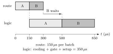
Routing and logic use independent resources in this illustrative schedule. Batch B finishes routing at $300\,\mu\mathrm{s}$ and waits in a buffer until logic is free at $500\,\mu\mathrm{s}$. Finite completion time includes filling the pipeline; routing conflicts or extra return operations would increase it.

For pure exponential dephasing with $T_2=10\,\mathrm{s}$ throughout this schedule, the coherence multiplier would be $\lambda=e^{-850\,\mu\mathrm{s}/T_2}$. The contrast loss is $1-\lambda\approx8.5\times10^{-5}$. The equivalent Pauli-$Z$ probability is $(1-\lambda)/2\approx4.25\times10^{-5}$, and the average gate infidelity of this idle dephasing channel is $(1-\lambda)/3$. These are different quantities. None includes entangling, transport, cooling, or measurement errors, and a stationary echoed coherence time need not describe an illuminated, moving qubit.

Exercises

1. Check a clock point

Suppose

$$\omega_q(B) = \omega_0+\beta(B-B_0)^2.$$

Find the first- and second-order magnetic sensitivities at $B_0$. What has and has not been protected?

Solution

Differentiating,

$$\frac{d\omega_q}{dB} = 2\beta(B-B_0),$$

so the first derivative vanishes at $B_0$. The curvature is

$$\frac{d^2\omega_q}{dB^2} = 2\beta.$$

The transition is first-order insensitive to magnetic fluctuations about the bias point, not independent of magnetic field. Quadratic magnetic noise, bias error, AC Stark shifts, oscillator phase noise, relaxation, and control errors remain.

2. Estimate a Lamb–Dicke parameter

A $^{40}\mathrm{Ca}^{+}$ ion has a mode frequency $\nu/(2\pi)=1.0\,\mathrm{MHz}$. A $729\,\mathrm{nm}$ beam is aligned with the mode, and take $b=1$. Estimate $x_0$ and $\eta=kx_0$.

Solution

Using $m\approx40(1.6605\times10^{-27}\,\mathrm{kg})$,

$$\begin{aligned} x_0 &= \sqrt{\frac{\hbar}{2m\nu}} \\ &\approx 1.12\times10^{-8}\,\mathrm m = 11.2\,\mathrm{nm}. \end{aligned}$$

The wave number is

$$k = \frac{2\pi}{729\,\mathrm{nm}} \approx 8.62\times10^6\,\mathrm{m}^{-1},$$

so

$$\eta \approx 0.097.$$

For a Raman transition one must use the projected wavevector difference, and for a multi-ion mode include the appropriate participation factor.

3. Infer a mean occupation

In the Lamb–Dicke and weak-excitation limits, the red-to-blue sideband strength ratio is

$$r = \frac{\bar n}{\bar n+1}.$$

Find $\bar n$ when $r=0.08$.

Solution

Solving for $\bar n$ gives

$$\bar n = \frac{r}{1-r} = \frac{0.08}{0.92} \approx 0.087.$$

For a weak probe of one ion and one resolved mode, red and blue probabilities are proportional to $\langle a^\dagger a\rangle$ and $\langle aa^\dagger\rangle$. Their ratio determines the mean for any motional state with finite occupation in the Lamb–Dicke regime; thermality is not required at this order. Comparable pulse strengths and negligible saturation are required. The ratio does not determine the full distribution or certify a temperature. Stronger pulses or collective excitation require the appropriate dynamical model.

4. Separate reachability from concurrency

A 20-ion register can implement a calibrated gate on any selected pair. How many pair edges are reachable? What is the maximum number of disjoint two-qubit gates in one abstract layer?

Solution

The complete pair graph has

$$\binom{20}{2} = \frac{20\cdot19}{2} = 190$$

edges. A disjoint matching can contain at most

$$\left\lfloor\frac{20}{2}\right\rfloor = 10$$

gates. Optical channels, shared modes, crosstalk, and pulse compatibility may reduce actual concurrency below ten. Thus 190 reachable pairs does not mean 190 simultaneous gates.

5. Quantify imperfect mode closure

Two spin branches finish a gate with relative mode displacement $|\Delta\alpha|=0.05$. If the mode has $\bar n=0.20$, estimate the thermal coherence factor

$$C = \exp\!\left[ -\left(\bar n+\frac12\right) |\Delta\alpha|^2 \right].$$

Solution

The exponent is

$$-\left(0.20+0.50\right)(0.05)^2 = -1.75\times10^{-3}.$$

Therefore

$$C \approx e^{-0.00175} \approx 0.99825.$$

The corresponding coherence loss is about $1.75\times10^{-3}$. This is only the contribution of the specified residual displacement and thermal mode, not the total entangling-gate infidelity.

6. Compare serial and pipelined QCCD schedules

Use $a=150\,\mu\mathrm{s}$ and $b=350\,\mu\mathrm{s}$ from the worked example. Find the empty-pipeline completion time for three batches and compare it with a serial schedule and the steady interval.

Solution

The first completion is at $a+b=500\,\mu\mathrm{s}$, followed by completions at 850 and $1200\,\mu\mathrm{s}$. Thus

$$T_3=150+350+2(350)=1200\,\mu\mathrm{s}.$$

Serial execution takes $3(150+350)=1500\,\mu\mathrm{s}$. The steady interval is $350\,\mu\mathrm{s}$, whereas the average time per batch in this three-batch run is $400\,\mu\mathrm{s}$. The difference is initial pipeline fill, even before adding physical conflicts or retries.

7. Estimate a photonic-link rate

For each arm of a two-photon link, take

$$\begin{aligned} p_{\mathrm{emit}}&=0.90, & \beta&=0.80, \\ \eta_{\mathrm{col}}&=0.15, & \eta_{\mathrm{path}}&=0.70, \\ \eta_{\mathrm{det}}&=0.80. \end{aligned}$$

Using $p_{\mathrm h}=p_\gamma^2/2$ and an attempt rate of $20\,\mathrm{kHz}$, estimate the heralding rate and mean waiting time.

Solution

One-arm success is

$$\begin{aligned} p_\gamma &= (0.90)(0.80)(0.15) \times (0.70)(0.80)\\ &= 0.06048. \end{aligned}$$

Thus

$$p_{\mathrm h} = \frac{(0.06048)^2}{2} \approx 1.83\times10^{-3}.$$

The idealized rate and waiting time are

$$\begin{aligned} R_{\mathrm h} &= (2.0\times10^4)p_{\mathrm h} \approx 36.6\,\mathrm{s}^{-1}, \\ \tau_{\mathrm{link}} &\approx 27.3\,\mathrm{ms}. \end{aligned}$$

Dead time, photon indistinguishability, detector acceptance windows, dark counts, and unsuccessful state-reset cycles can reduce the useful rate.

8. Bound measurement crosstalk

During one ancilla measurement, suppose each of 15 spectator ions has an independent probability $c=2\times10^{-4}$ of an unwanted optical-pumping event. Estimate the probability that at least one spectator is affected.

Solution

Under the stated independence model,

$$\begin{aligned} p_{\ge1} &= 1-(1-c)^{15} \\ &\approx 1-(0.9998)^{15} \approx 3.0\times10^{-3}. \end{aligned}$$

That is about $0.30\%$ per ancilla measurement. Repeated rounds can make the aggregate risk important. Shared scattering or beam leakage would violate the independence assumption and requires a correlated-error measurement.

References

• R. Bowler et al., “Coherent diabatic ion transport and separation in a multizone trap array,” Physical Review Letters 109, 080502 (2012), doi:10.1103/PhysRevLett.109.080502.
• K. R. Brown et al., “Materials challenges for trapped-ion quantum computers,” Nature Reviews Materials 6, 892–905 (2021), doi:10.1038/s41578-021-00292-1.
• C. D. Bruzewicz, J. Chiaverini, R. McConnell, and J. M. Sage, “Trapped-ion quantum computing: Progress and challenges,” Applied Physics Reviews 6, 021314 (2019), doi:10.1063/1.5088164.
• J. I. Cirac and P. Zoller, “Quantum computations with cold trapped ions,” Physical Review Letters 74, 4091–4094 (1995), doi:10.1103/PhysRevLett.74.4091.
• H. Häffner, C. F. Roos, and R. Blatt, “Quantum computing with trapped ions,” Physics Reports 469, 155–203 (2008), doi:10.1016/j.physrep.2008.09.003.
• T. P. Harty et al., “High-fidelity preparation, gates, memory, and readout of a trapped-ion quantum bit,” Physical Review Letters 113, 220501 (2014), doi:10.1103/PhysRevLett.113.220501.
• D. Hucul et al., “Modular entanglement of atomic qubits using photons and phonons,” Nature Physics 11, 37–42 (2015), doi:10.1038/nphys3150.
• D. Kielpinski, C. Monroe, and D. J. Wineland, “Architecture for a large-scale ion-trap quantum computer,” Nature 417, 709–711 (2002), doi:10.1038/nature00784.
• D. Leibfried, R. Blatt, C. Monroe, and D. Wineland, “Quantum dynamics of single trapped ions,” Reviews of Modern Physics 75, 281–324 (2003), doi:10.1103/RevModPhys.75.281.
• K. K. Mehta et al., “Integrated optical multi-ion quantum logic,” Nature 586, 533–537 (2020), doi:10.1038/s41586-020-2823-6.
• C. Monroe et al., “Large-scale modular quantum-computer architecture with atomic memory and photonic interconnects,” Physical Review A 89, 022317 (2014), doi:10.1103/PhysRevA.89.022317.
• I. D. Moore, W. C. Campbell, E. R. Hudson, M. J. Boguslawski, D. J. Wineland, and D. T. C. Allcock, “Photon scattering errors during stimulated Raman transitions in trapped-ion qubits,” Physical Review A 107, 032413 (2023), doi:10.1103/PhysRevA.107.032413.
• R. Ozeri et al., “Errors in trapped-ion quantum gates due to spontaneous photon scattering,” Physical Review A 75, 042329 (2007), doi:10.1103/PhysRevA.75.042329.
• J. M. Pino et al., “Demonstration of the trapped-ion quantum CCD computer architecture,” Nature 592, 209–213 (2021), doi:10.1038/s41586-021-03318-4.
• A. Sørensen and K. Mølmer, “Entanglement and quantum computation with ions in thermal motion,” Physical Review A 62, 022311 (2000), doi:10.1103/PhysRevA.62.022311.
• S. Srinivas et al., “High-fidelity laser-free universal control of trapped ion qubits,” Nature 597, 209–213 (2021), doi:10.1038/s41586-021-03809-4.