Modular Architectures

A modular quantum architecture builds a larger machine from smaller quantum systems connected by quantum interactions and classical controls. The connections may transfer a state, create shared entanglement, transport an atom, or perform a joint measurement. Useful scaling depends on how often these operations are available, how long data must wait, and which errors can affect several modules together.

Smaller units can simplify fabrication, calibration, and replacement, but remote operations add noise, latency, and competition for shared resources. This page develops those physical tradeoffs. Distributed Quantum Computing develops program partitioning and remote-gate protocols; Quantum Network Architectures treats networks serving multiple users.

Required background. Hardware Overview introduces device components; Interconnects and Transduction describes transfer and conversion channels; Quantum Memories explains storage noise; Quantum Teleportation shows how shared entanglement and classical messages transfer an unknown state.

Quantum modules and their connections

A module is a chosen physical subsystem, not a fixed qubit count or distance. It might be a trap zone, superconducting die, cavity register, photonic subsystem, or separated node. State which meaning is intended: transport between two zones inside one vacuum chamber and an optical link between separate chambers create different constraints.

A module can share external clocks, lasers, cooling, or controllers. These dependencies do not make it cease to be a module, but they can limit parallel operation and create shared failures. The quantum interaction graph and the graph of shared classical or environmental resources generally differ.

Data and communication roles

Data qubits store the computational state. Communication qubits couple to a link, while memories and ancillas protect information and support local operations. One device can serve several roles at different times, but it cannot be assumed available for all of them simultaneously.

For example, repeated optical excitation of a communication spin can disturb a nearby memory even when every failed link attempt is correctly heralded. A transmon emitting a photon may be unavailable for another gate. A photonic delay line provides storage with a fixed delay and loss, rather than an arbitrarily addressable memory.

Connection	What crosses the boundary	Main constraint
Direct coherent transfer	An unknown state in a carrier or propagating mode	Loss and capture errors act on the data itself
Heralded entanglement	A prepared shared resource followed by a success message	Random production time and errors in accepted pairs
Teleported gate	Shared entanglement consumed with local operations and messages	Memory, local errors, and feed-forward dependencies
Matter transport	The physical qubit carrier	Motion, cooling, loss, and occupied transport paths
Joint measurement or fusion	A parity outcome or connection between resource states	Detector efficiency, known failure outcomes, and consumed states

The same photon can support several of these operations. Classify a connection by its action on the input state. An attempted transfer on every clock cycle need not be an accurate identity channel. A heralded failure may reveal that data were lost; it does not automatically leave them intact. Likewise, a failed fusion can consume photons or alter the remaining graph state, depending on the protocol.

For an ideal gate-teleportation protocol, a usable entangled resource makes the subsequent local measurement and correction sequence deterministic. Creating that resource can still require many trials. Gottesman and Chuang develop this separation between resource preparation and gate execution; the hardware demonstrations discussed below test particular implementations.

Why divide a processor into modules?

Smaller repeated units may be easier to screen and replace than one large all-required device. The gain depends on connector yield, defect correlations, and the ability to operate with missing parts, as explained in Materials and Fabrication. Dividing a register may reduce spectral crowding and control complexity, while increasing the number of controllers and synchronization problems.

Specialization can also help: a long-lived memory need not be the fastest emitter, and a resource-state factory need not sit beside every data qubit. Its benefit depends on the write, transfer, and read costs of the complete path. A superior isolated memory can be ineffective behind a lossy interface.

Runtime follows the critical path of a schedule. Local gates, resource generation, and classical processing may overlap, so their total durations should not always be added. Conversely, a small number of remote gates can dominate runtime when every one waits for a slow link or an occupied port.

Capacity, topology, and simultaneous operation

Let $G=(V,E)$ describe permitted connections. Choose one resource unit, such as a usable elementary Bell pair of a specified quality; do not add rates of Bell pairs, transfers, and fusions without a conversion model. Let $c_e$ be an edge’s available rate in those units under a stated schedule.

For pair-swapping and routing protocols in which each delivered pair needs at least one elementary pair across a cut $S$, define

$$C(S)=\sum_{e\in\delta(S)}c_e.$$

Sustained cross-cut demand cannot exceed the achievable supply. In a deterministic fluid model, with no initial stored entanglement and a fixed capacity bound, a batch requiring $B(S)$ crossing resources obeys

$$T\ge\max_S\frac{B(S)}{C(S)}.$$

If $c_e$ denotes only a stochastic mean rate, this expression is instead a throughput estimate, not a hard lower bound on every completion time. Initial stock, distillation, failed swapping, or a different distributed protocol changes the resource calculation. A small finite batch can also finish faster or slower than its mean-rate estimate.

Reachability does not establish parallel capacity

An edge rate measured with all other links idle may be unattainable when several links operate. A shared switch, bus, detector bank, or single communication qubit imposes additional constraints.

For example, three modules form a triangle, each with one communication port. Every edge can deliver $1000$ pairs per second when used alone, but no two edges can operate together because they share a vertex. The entire triangle therefore produces at most $1000$ pairs per second. Demands of $500$ pairs per second on each edge pass the naive cut tests using isolated edge rates, yet require an impossible total of $1500$ pairs per second.

The correct capacities come from time-sharing compatible sets of active edges. Cut bounds are useful necessary constraints within their resource model; they do not by themselves prove that a multicommodity schedule exists. Switching time and recalibration can further reduce the available time.

Partitioning and bursts

For a circuit interaction graph and a partition $\pi$ into modules, a simple cost is

$$C_{\mathrm{cut}}(\pi)=\sum_{(a,b)} w_{ab}\,\mathbf1[\pi(a)\ne\pi(b)].$$

This counts weighted interactions crossing modules. It does not include edge rates, memory occupancy, or concurrent local work. A schedule with few remote gates can still create a large burst of requests at a logical measurement or resource-injection step. Qubit Mapping and Routing develops the compiler problem; here the hardware must supply the assumed simultaneous operations.

Probabilistic links and memory during retries

Suppose $M$ independent modes are attempted in a round of duration $\tau$, and each succeeds with probability $p$. Then

$$\begin{aligned} K&\sim\operatorname{Binomial}(M,p),\\ P(K\ge1)&=1-(1-p)^M,\\ \mathbb E[K]&=Mp. \end{aligned}$$

These last two quantities answer different questions. If the receiver can retain at most one raw pair, its raw supply is $P(K\ge1)/\tau$. If all successes can be stored independently, the mean raw count rate is $Mp/\tau$. Temporal modes count toward $M$ only when they fit inside the stated round and the hardware can preserve their independent attempts and outcomes.

The round duration must include blocking reset, preparation, and herald latency. Additional downtime is not a dimensionless rejection fraction. Distillation consuming several raw pairs needs an input-to-output resource calculation as well as a success probability. Shared emitters, detector dead time, and correlated drift can invalidate the binomial model.

For independent rounds with accepted success probability $p_a$ and one output at most per round, the number $N$ of rounds through success is geometric:

$$P(N>n)=(1-p_a)^n,\qquad \mathbb E[N]=\frac1{p_a}.$$

Even when the mean time $\tau/p_a$ is acceptable, the tail can violate a memory deadline. Failed attempts may also disturb stored data through scattered light, heating, or shared control. This disturbance must be measured under the attempt sequence, not inferred from an idle-memory lifetime.

Pair age and request latency are different

A pair prepared ahead of demand ages in memory until it is consumed. A request for a pair that does not yet exist instead waits for generation. The waiting data can decohere, but the newly created pair has not aged for the full request latency. Stocking pairs ahead of demand trades latency for storage noise and limited memory occupancy.

For an initially ideal Bell pair under independent pure dephasing, let the single-memory coherences decay as $e^{-\gamma_A t}$ and $e^{-\gamma_B t}$. Then

$$c(t)=e^{-(\gamma_A+\gamma_B)t}, \qquad F_{\Phi^+}(t)=\frac{1+c(t)}2.$$

Here $F$ is the squared state fidelity, equal to the overlap with the pure target. The coherence factor is neither the Bell fidelity nor a survival probability. Relaxation, leakage, and phase-reference errors change this channel model.

An explicit request-queue model

Consider one server generating pairs on demand, serving requests in first-come, first-served order. Assume independent Poisson requests at rate $\lambda$, independent exponential service times of rate $\mu$, infinite waiting space, no abandonment, and no stored inventory. This is the $M/M/1$ model discussed by Harchol-Balter. It has a stationary queue only for $\lambda<\mu$.

In stationarity, the full response time $W$, including waiting and service, has

$$\begin{aligned} P(W>w)&=e^{-(\mu-\lambda)w},\\ \mathbb E[W]&=\frac1{\mu-\lambda}. \end{aligned}$$

This particular exponential distribution uses first-come, first-served service. It is not a general consequence of knowing two mean rates. Real factories have finite memories, different request classes, setup times, and resource expiry. A finite queue can stay bounded even under overload by rejecting requests; bounded queue length alone then says little about delivered service.

Suppose already-existing data lose coherence by $e^{-w/T}$ while awaiting their resource, independently of the queue trajectory apart from elapsed time. Average over the latency distribution:

$$\begin{aligned} \mathbb E[e^{-W/T}] &=\int_0^\infty e^{-w/T}(\mu-\lambda)e^{-(\mu-\lambda)w}\,dw\\ &=\frac{\mu-\lambda}{\mu-\lambda+T^{-1}}. \end{aligned}$$

Substituting the mean latency gives $e^{-\mathbb E[W]/T}$, a different quantity. Convexity makes it no larger than the true average here. Neither one bounds the worst request: use the latency tail for deadline questions.

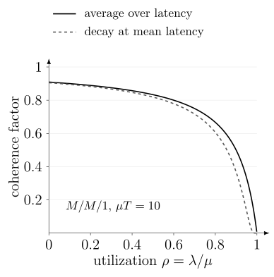
For $\mu T=10$, the solid curve averages $e^{-W/T}$ over the response-time distribution; the dashed curve evaluates decay at the mean time. At $\rho=\lambda/\mu=0.95$, they give $1/3$ and $e^{-2}\simeq0.135$. This model describes data waiting for a resource, not the storage age of a pair generated at the end of the wait.

Worked example: multiplexing followed by a request queue

Take $M=16$, $p=2\times10^{-4}$, and $\tau=2\,\mu\mathrm s$. Select at most one raw success per round, and accept that selected pair independently with probability $q=0.70$, with no added blocking time. Then

$$\begin{aligned} p_a&=q[1-(1-p)^{16}]\simeq0.002237,\\ \mu&=p_a/\tau\simeq1118.3\,\mathrm{s}^{-1}. \end{aligned}$$

This selection rule differs from accepting every mode independently and then keeping any accepted one, whose success probability would be $1-(1-pq)^M$. Keeping all accepted modes gives yet another output count.

For rare per-round successes, approximate the geometric service time by an exponential. With Poisson demand $\lambda=800\,\mathrm{s}^{-1}$, the resulting $M/M/1$ model gives

$$\rho\simeq0.715,\qquad \mathbb E[W]\simeq3.14\,\mathrm{ms}.$$

For data coherence time $T=50\,\mathrm{ms}$,

$$\begin{aligned} \mathbb E[e^{-W/T}]&\simeq0.9409,\\ e^{-\mathbb E[W]/T}&\simeq0.9391,\\ P(W>10\,\mathrm{ms})&\simeq0.0415. \end{aligned}$$

The two averages happen to be close here, while about four percent of requests exceed ten milliseconds. This is an illustrative queue model, not a remote-gate fidelity: it omits the pair state, local operations, feed-forward, and attempt-induced disturbance beyond the specified decay.

Remote-operation errors and classical messages

Let $E_j$ be specified stochastic fault events in pair preparation, local gates, measurement, waiting, or control. If every operation failure requires at least one such event, the union bound gives

$$\begin{aligned} P(\text{failure})&\le P\!\left(\bigcup_j E_j\right) \\ &\le\sum_jP(E_j). \end{aligned}$$

Independence is unnecessary for this bound. Under independence, $P(\bigcup_jE_j)=1-\prod_j(1-p_j)$, whose leading small-error term is the sum. Fault occurrence and final logical failure need not coincide: faults can be detected, corrected, or cancel.

Average gate infidelity is not generally the probability of a stochastic fault event. Coherent phase errors can accumulate differently from random Pauli errors; leakage and conditioning can change the effective state space. Use the channel definitions in Metrics for Quantum Hardware when composing those operations. Conditional pair fidelity also omits discarded attempts and their effect on the data.

Phase references and feed-forward

A pair with a known phase can be corrected or interpreted in a corresponding frame. If instead the unrecorded phase varies between trials,

$$|\Phi_\phi\rangle=\frac{|00\rangle+e^{i\phi}|11\rangle}{\sqrt2}$$

has ensemble overlap

$$\overline F_{\Phi^+}=\frac{1+\operatorname{Re}\mathbb E[e^{i\phi}]}2.$$

Zero-mean Gaussian phase noise of variance $\sigma_\phi^2$ gives $(1+e^{-\sigma_\phi^2/2})/2$. Each individual pair is maximally entangled, but an unknown phase makes the ensemble less useful relative to a fixed target. Reference stability depends on the protocol; path motion, converter pump phase, and clock drift need not enter all encodings in the same way.

Classical messages must associate an outcome with the right memory and operation. Pauli-frame tracking can defer physical corrections through Clifford operations, but an adaptive non-Clifford step or output interpretation can require the pending bits. Message acquisition, classification, transport, queueing, and actuation all contribute to the relevant deadline. Timing only the classifier misses these dependencies.

Error correction across module boundaries

A code block can span physical modules, or each module can hold a complete logical qubit linked by encoded operations. These arrangements impose different requirements on pairs, memories, local gates, and syndrome timing.

Nickerson, Li, and Benjamin and later Nickerson, Fitzsimons, and Benjamin analyzed cells connected by noisy photonic links. Purification and distributed stabilizer measurements can tolerate links noisier than local operations, at a cost in raw pairs, local work, and time. Their thresholds are conditional on the specified noise model, cell resources, schedule, and decoder. They are not universal fidelity requirements for arbitrary modular hardware.

When a stabilizer waits for a random resource, missing or delayed checks alter the syndrome history. The decoder needs the actual time and location of the check, along with heralded loss or leakage information. Replacing all of this by one average depolarizing rate can hide correlated faults and discard useful flags. A successful failure herald does not by itself correct an unknown state that was destroyed.

The relevant scaling test increases code size or protection while retaining the link generation, waiting, control, and decoder costs. A small error- detecting experiment need not demonstrate logical error suppression. Surface Code and Quantum LDPC Codes explain the codes; this hardware question concerns how their checks are realized.

Shared failures and replaceable hardware

At a specified instant, independent module availabilities $A_i$ give $A_{\mathrm{series}}=\prod_iA_i$ when every module is required. For one thousand modules with $A_i=0.999$, this is about $0.368$. It is an availability calculation, not a first-failure survival probability.

Spares can help if routing and encoding tolerate the missing module. A shared controller or cooling system remains a common cause: if it is required and has availability $A_c$, the complete machine’s availability cannot exceed $A_c$. Under independence between that infrastructure and the remaining subsystems, multiply the subsystem availability by $A_c$.

Replacement also takes time for cooling, alignment, calibration, and verification. Mechanical compatibility does not ensure matching frequencies, couplings, or optical modes. Most importantly, a new physical module does not restore an unknown state lost in the old one. Encoded recovery, prior teleportation, or another state-preserving protocol must supply that function; the no-cloning theorem excludes a generic classical backup.

Physical examples of modularity

Ion transport. Kielpinski, Monroe, and Wineland proposed the quantum charge-coupled-device approach, and Pino and colleagues demonstrated a processor with transport between zones. Junction contention, heating, and cooling are the relevant connection costs; this is different from a photonic link between separate traps.

Photonic links between matter registers. Hucul and colleagues combined local phonon-mediated gates with remote photon-mediated entanglement. Main and colleagues used separate network and circuit qubits to perform repeated teleported gates between two ion modules. The distinction is operational: the second type of experiment tests a sequence of remote operations and memory during retries, beyond producing one entangled pair.

Superconducting modes and dies. Microwave buses and propagating photons connect circuit modules. Chou and colleagues teleported a gate between two cavity-encoded qubits; Burkhart and colleagues demonstrated error-detected state transfer. These examples distinguish encoded operations and detected loss from an assertion that arbitrary module replacement preserves data.

Photonic and heterogeneous systems. Sources, switches, delays, detectors, and matter memories can be separate subsystems. Loss and mode matching accumulate across their interfaces. Photonic Qubits and Interconnects and Transduction develop the physical mechanisms. Detailed experimental comparisons belong with Network Case Studies; current scaling questions are collected in Modular and Networked Quantum Computers.

Exercises

1. Classify boundary services

For each case, identify the primary boundary service: (a) an ion is shuttled from a memory zone to a gate zone, (b) photons are detected until two remote memories are heralded entangled, (c) a microwave wave packet carrying an unknown cavity state is captured by another module, and (d) two photonic graph states are joined by a probabilistic measurement.

Solution

(a) is transported matter. (b) is heralded entanglement. (c) is direct coherent state transfer; the statement alone does not establish whether success is deterministic or heralded. (d) is fusion or joint measurement. The same physical carrier, especially a photon, can support different services; the operational input and output define the classification.

2. A cut-capacity lower bound

Four modules form a line $A$–$B$–$C$–$D$. The edge capacities are $c_{AB}=1000$, $c_{BC}=300$, and $c_{CD}=800$ accepted pairs per second. A batch requires $6000$ pairs from modules on the left of the $B$–$C$ cut to modules on the right. Assume no stored cross-cut entanglement, one elementary pair consumed per crossing, and constant deterministic fluid capacities. Find the communication-time lower bound.

Solution

Every required pair must cross the $B$–$C$ edge, so

$$T_{\mathrm{boundary}} \ge \frac{6000}{300\,\mathrm{s}^{-1}} = 20\,\mathrm{s}.$$

The faster outer edges cannot remove the middle cut bottleneck. Contention and local operations can only increase completion time beyond this bound. If the quoted capacities are instead stochastic mean rates, 20 seconds is a throughput estimate, not a lower bound on every realization.

3. Multiplexing gain

A heralded link has per-mode success probability $p=10^{-3}$ and attempts $M=100$ independent modes each round.

1. Find the probability of at least one success.
2. Compare it with the approximation $Mp$.
3. If all successful modes can be stored independently, what is the mean number of pairs per round?

Solution

The exact probability is

$$p_{\mathrm{eff}} = 1-(1-10^{-3})^{100} \approx 0.0952.$$

The linear approximation gives $Mp=0.1$, about five percent too high. It is valid when $Mp\ll1$ and shared constraints are absent. It eventually fails as a probability approximation because a probability cannot exceed one. However, $\mathbb E[K]=Mp=0.1$ remains the exact mean pair count for the independent-binomial model when all successes are retained. Actual hardware may share emitters, detectors, switching, bandwidth, or reset.

4. Queue stability and burst margin

An entanglement factory supplies accepted pairs at mean rate $\mu=2000\,\mathrm{s}^{-1}$. Two workloads demand $900\,\mathrm{s}^{-1}$ and $850\,\mathrm{s}^{-1}$.

1. Does the load satisfy the stability condition for an ideal infinite-buffer $M/M/1$ request queue?
2. What fraction of capacity remains?
3. Why can the system still miss deadlines?

Solution

The total demand is

$$\lambda = 900+850 = 1750\,\mathrm{s}^{-1} < \mu,$$

so this specified $M/M/1$ model has a stationary request queue. Mean rates alone do not establish stability for an arbitrary scheduler and resource network. The unused mean capacity is $250\,\mathrm{s}^{-1}$, or $12.5\%$ of supply. Bursts, correlated generation failures, finite buffers, quality rejection, priority traffic, and pair expiry can still produce long tails and missed deadlines.

5. Pair-age acceptance

Under pure dephasing, a stored Bell pair has coherence factor $\eta(t)=e^{-t/T}$ with combined two-memory coherence time $T=20\,\mathrm{ms}$. A protocol requires $\eta\ge0.90$. Find the maximum accepted age.

Solution

Solve

$$e^{-t/T} \ge 0.90.$$

Thus

$$\begin{aligned} t &\le -T\ln(0.90) \\ &\approx 2.11\,\mathrm{ms}. \end{aligned}$$

For this channel the Bell fidelity is $F=(1+\eta)/2$, so the specified coherence condition is $F\ge0.95$, not $F\ge0.90$. Other error channels need more than a single dephasing factor.

6. Partition a circuit graph

Six logical qubits form two triangles, $(1,2,3)$ and $(4,5,6)$, with one repeated interaction between qubits $3$ and $4$. Two modules each hold three qubits. Compare the partitions $\{1,2,3\}|\{4,5,6\}$ and $\{1,2,4\}|\{3,5,6\}$ under equal edge weights.

Solution

The first partition cuts only edge $(3,4)$, so its cut cost is one. The second cuts triangle edges $(1,3)$ and $(2,3)$, triangle edges $(4,5)$ and $(4,6)$, and edge $(3,4)$, since $3$ and $4$ lie in different modules. Its cut cost is five.

The first partition is therefore better under the simple objective. A real mapping could differ if one module has a failed qubit, edge capacities are unequal, or concurrent local gates dominate.

7. Combining stochastic faults

A remote gate has independent small-error estimates $p_{\mathrm{pair}}=0.006$, two local contributions of $0.001$ each, $p_{\mathrm{meas}}=0.002$, and $p_{\mathrm{wait}}=0.003$. Estimate the first-order failure probability and state the model’s limitation.

Solution

If these are probabilities of specified fault events, their sum gives the union bound

$$\begin{aligned} &P(\text{at least one fault}) \\ &\quad\le0.006+2(0.001)+0.002+0.003 \\ &\quad=0.013. \end{aligned}$$

The bound does not require independence. Under the additional independence assumption, the exact probability of at least one fault is

$$\begin{aligned} &1-(1-0.006)(1-0.001)^2 \times(1-0.002)(1-0.003)\\ &\quad\simeq0.01294. \end{aligned}$$

An operation fails only if the faults produce an uncorrected logical effect; several faults can cancel or be detected. Average gate infidelities are not automatically probabilities of such events, so their sum is not this bound.

8. Availability with and without a spare

Four independent modules each have availability $A=0.99$.

1. Find availability if all four are required.
2. Suppose the architecture installs five identical modules and works whenever at least four are available. Find the idealized availability.

Solution

With all four required,

$$A_{\mathrm{series}} = 0.99^4 \approx 0.9606.$$

With one spare, the system works with exactly four or all five modules:

$$\begin{aligned} A_{\ge4} &= \binom54(0.99)^4(0.01) + (0.99)^5 \\ &\approx 0.9990. \end{aligned}$$

This optimistic gain assumes independent failures, instant rerouting, a truly interchangeable spare, and no requalification delay. It also assumes the encoded information can survive a missing module; replacing hardware does not reconstruct an unprotected unknown quantum state.

9. What simulations and experiments establish

A paper simulates a distributed surface code under a fitted link-noise model and reports a threshold. Another experiment creates one Bell pair across two modules. Which claims are justified?

Solution

The first is a hardware-informed simulation result: it establishes a conditional threshold within the code, noise, timing, and decoder model. It does not demonstrate hardware below threshold.

The second is an experimental remote-entanglement demonstration under the reported acceptance and measurement conditions. It does not establish distributed computation, queue stability, error correction, or scaling. Both results can be important without establishing those additional capabilities.

10. Test repeated remote operations

Propose a benchmark that goes beyond one remote Bell pair but remains feasible for two small modules.

Solution

One useful benchmark is a repeated remote parity measurement or teleported two-qubit gate while each module stores an independent spectator state. Measure:

• an input ensemble for process reconstruction or randomized validation;
• accepted and unconditional success metrics;
• pair-attempt, accepted-operation, and wall-clock rates;
• spectator-memory error during retries;
• classical latency and timeout policy;
• repeated operation depth;
• calibration age, drift interval, and uncertainty.

Compare against the same local operation when possible. Repeat enough times to measure tails and drift, then test a two-module encoded primitive or small distributed circuit. This tests useful operation and its effect on stored data; a separate scaling study is needed to establish fault tolerance.

11. Average coherence from a queue

For the stationary first-come, first-served $M/M/1$ model, an arriving request finds $n$ requests in the system with probability $(1-\rho)\rho^n$. Its response time then sums $n+1$ exponential service times of rate $\mu$. Find $\mathbb E[e^{-sW}]$ and set $s=1/T$.

Solution

An exponential service time has Laplace transform $\mu/(\mu+s)$. Conditional independence and the geometric series give

$$\begin{aligned} \mathbb E[e^{-sW}] &=\sum_{n=0}^\infty(1-\rho)\rho^n \left(\frac{\mu}{\mu+s}\right)^{n+1}\\ &=\frac{\mu-\lambda}{\mu-\lambda+s}. \end{aligned}$$

At $s=1/T$ this is the averaged coherence factor. At $\mu T=10$ and $\rho=0.95$, it equals $1/3$, whereas decay at the mean latency is $e^{-2}\simeq0.135$. This calculation concerns a stationary arrival, not an initially empty queue or stored-pair age.

12. A shared-port bottleneck

Three modules form a triangle, each with one communication port. Each edge produces $1000$ pairs per second when active. In a deterministic fluid model, how long does producing 120 pairs on each of the three edges take? Neglect switching time and assume the outputs can be moved to adequate separate storage.

Solution

Every two edges share a port, so only one can operate at once. The total active time is at least $3(120)/1000=0.36\,\mathrm s$, achieved by using each edge for $0.12\,\mathrm s$. Naively summing isolated edge capacities at every cut would give only $240/2000=0.12\,\mathrm s$. That cut bound misses the shared-port constraint and is not achievable.

References

• L. D. Burkhart et al., “Error-detected state transfer and entanglement in a superconducting quantum network,” PRX Quantum 2, 030321 (2021), doi:10.1103/PRXQuantum.2.030321.
• K. S. Chou et al., “Deterministic teleportation of a quantum gate between two logical qubits,” Nature 561, 368–373 (2018), doi:10.1038/s41586-018-0470-y.
• D. Gottesman and I. L. Chuang, “Demonstrating the viability of universal quantum computation using teleportation and single-qubit operations,” Nature 402, 390–393 (1999), doi:10.1038/46503.
• M. Harchol-Balter, Performance Modeling and Design of Computer Systems: Queueing Theory in Action (Cambridge University Press, 2013), author’s book page.
• D. Hucul et al., “Modular entanglement of atomic qubits using photons and phonons,” Nature Physics 11, 37–42 (2015), doi:10.1038/nphys3150.
• L. Jiang, J. M. Taylor, A. S. Sørensen, and M. D. Lukin, “Distributed quantum computation based on small quantum registers,” Physical Review A 76, 062323 (2007), doi:10.1103/PhysRevA.76.062323.
• D. Kielpinski, C. Monroe, and D. J. Wineland, “Architecture for a large-scale ion-trap quantum computer,” Nature 417, 709–711 (2002), doi:10.1038/nature00784.
• D. Main et al., “Distributed quantum computing across an optical network link,” Nature 638, 383–388 (2025), doi:10.1038/s41586-024-08404-x.
• C. Monroe et al., “Large-scale modular quantum-computer architecture with atomic memory and photonic interconnects,” Physical Review A 89, 022317 (2014), doi:10.1103/PhysRevA.89.022317.
• M. A. Nielsen and I. L. Chuang, Quantum Computation and Quantum Information, 10th anniversary ed. (Cambridge University Press, 2010).
• N. H. Nickerson, J. F. Fitzsimons, and S. C. Benjamin, “Freely scalable quantum technologies using cells of 5-to-50 qubits with very lossy and noisy photonic links,” Physical Review X 4, 041041 (2014), doi:10.1103/PhysRevX.4.041041.
• N. H. Nickerson, Y. Li, and S. C. Benjamin, “Topological quantum computing with a very noisy network and local error rates approaching one percent,” Nature Communications 4, 1756 (2013), doi:10.1038/ncomms2773.
• J. M. Pino et al., “Demonstration of the trapped-ion quantum CCD computer architecture,” Nature 592, 209–213 (2021), doi:10.1038/s41586-021-03318-4.
• R. Van Meter, Quantum Networking (Wiley, 2014), doi:10.1002/9781118648919.