Network Case Studies

A quantum network must preserve quantum information while photons are lost, memories wait, and measurement outcomes travel between nodes. Four examples make these demands concrete: entanglement swapping, memory-assisted links, gates between processors, and satellite distribution. The central question in each case is what becomes usable at the end, and with what probability, quality, and delay.

Helpful background. Teleportation explains why shared entanglement and classical communication can transfer a state; entanglement swapping explains how two links become one; quantum memories explains storage and retrieval.

Entanglement across three nodes

Imagine Alice and Bob sharing one Bell pair, while Bob and Charlie share another. Bob holds two qubits. A Bell measurement on those qubits, followed by communicating its outcome, leaves Alice and Charlie with a known Bell state after an appropriate Pauli correction. Their qubits need never have interacted directly. The measurement consumes both elementary pairs: the network must prepare new resources for the next use.

Pan and colleagues demonstrated this idea with two polarization-entangled photon pairs in 1998. A joint measurement on one photon from each pair selected entanglement between the other two. This establishes the swapping mechanism; it does not by itself provide a stored pair that a user can request and consume later. Pan et al. (1998)

Storage changes the experiment. Pompili and colleagues used three diamond-spin nodes with optical links, local quantum logic, and real-time control to distribute multipartite entanglement and perform entanglement swapping. A memory holds the first successful link while the other link is attempted. Pompili et al. (2021)

Hermans and colleagues then teleported qubits between the non-neighboring endpoints of a three-node network. They first prepared and heralded the shared resource, then introduced the input state. For six cardinal qubit states, a selected-outcome protocol achieved mean fidelity $0.702(11)$ at one event per $117\,\mathrm{s}$. A version accepting every teleportation outcome after resource preparation achieved $0.688(10)$ at one event per $100\,\mathrm{s}$. Parentheses denote uncertainty in the final digits. “Every outcome” applies after the resource is ready; preparing that resource remains probabilistic. Hermans et al. (2022)

The familiar $2/3$ classical teleportation bound concerns an unknown qubit with a specified input ensemble and averaging rule. For a trace-preserving qubit channel, the equally weighted six cardinal states reproduce the uniform Bloch-sphere average. State-dependent acceptance can change the sampled ensemble, so conditional fidelities need their acceptance rule as well as a number. See quantum memory benchmarks for this distinction.

Waiting for two elementary links

Consider a deliberately simple memory-assisted model. Two independent links attempt entanglement in parallel. Each succeeds with fixed probability $p$ per cycle of duration $\tau$, including the time to learn the heralding result. Successful links stop attempting; there is no timeout. If $N_1,N_2$ are geometric waiting times starting at one cycle, then

$$\begin{aligned} T_{\rm ready}&=\tau\max(N_1,N_2),\\ A&=\tau|N_1-N_2|. \end{aligned}$$

Here $A$ is the extra storage age of the earlier link. It is not the time until both links are ready. The repeater waiting-time calculation gives

$$\begin{aligned} \mathbb E[T_{\rm ready}]&=\tau\frac{3-2p}{p(2-p)},\\ \mathbb E[A]&=\tau\frac{2(1-p)}{p(2-p)}. \end{aligned}$$

At $p=0.01$ and $\tau=0.10\,\mathrm{ms}$, the mean ready time is $14.97\,\mathrm{ms}$ and the mean extra storage age is $9.95\,\mathrm{ms}$. Sequential preparation would instead take $2\tau/p=20\,\mathrm{ms}$ on average. Parallel preparation saves time but requires two simultaneously usable links.

Suppose the relevant stored coherence decays as $C(A)=e^{-A/T_2}$. This is an effective single decay factor for the stored link, not automatically the coherence time of either isolated qubit. To predict its average value, average over the random age. With $q=1-p$ and $z=e^{-\tau/T_2}$,

$$\overline C=\frac{p}{2-p} \left(1+\frac{2qz}{1-qz}\right).$$

For $T_2=20\,\mathrm{ms}$, this gives $\overline C=0.6678$. Substituting the mean age into the exponential instead gives $0.6081$. Short waits contribute relatively high coherence, and the exponential is convex; therefore $\mathbb E[e^{-A/T_2}]\ge e^{-\mathbb E[A]/T_2}$. Neither number includes extra delays after both links become ready.

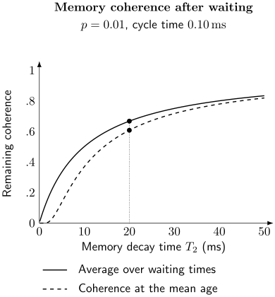
Calculated two-link example with $p=0.01$ and $\tau=0.10\,\mathrm{ms}$. The solid curve averages over all waiting times; the dashed curve uses their mean. The dots mark $T_2=20\,\mathrm{ms}$. There is no timeout, and link attempts are independent.

A timeout discards old pairs and changes both the age distribution and the completion rate. It can improve the quality of accepted pairs while increasing retries. Memory-assisted repeaters must balance those effects; other repeater architectures, including all-photonic designs, use different resources and need not contain long-lived matter memories.

What a long fiber link demonstrates

Knaut and colleagues entangled nuclear-spin memories using frequency conversion between visible light and the telecom band. They tested fiber spools up to $40\,\mathrm{km}$ and a $35\,\mathrm{km}$ deployed fiber loop. The latter ran out to an off-site location and back; its length is not a $35\,\mathrm{km}$ physical separation of the memory nodes. This is a remote-memory link, an ingredient for a repeater. Connecting two independently prepared links and delivering their endpoint state is an additional experiment. Knaut et al. (2024)

Turning shared entanglement into a remote gate

For distributed computation, the useful output is a gate on circuit qubits. A typical sequence is to herald a Bell resource on communication qubits, couple those qubits locally to circuit qubits, measure the communication qubits, and apply outcome-dependent corrections. Classical messages remain necessary. The Bell resource is consumed, while the circuit’s quantum information stays in the processors.

Main and colleagues demonstrated this sequence between trapped-ion modules about $2\,\mathrm{m}$ apart. Each module contained one $^{88}\mathrm{Sr}^{+}$ ion and one $^{43}\mathrm{Ca}^{+}$ ion; internal states of the calcium ion provided circuit and auxiliary degrees of freedom. The experiment reported a teleported controlled-$Z$ gate with $86.2(9)\%$ average gate fidelity and distributed Grover search with $71\%$ success. Its average entanglement generation rate, including interleaved cooling, was $9.7\,\mathrm{s}^{-1}$. Main et al. (2025)

These quantities answer different questions:

Quantity	What it describes	What else matters
Bell-pair rate	Available shared resources per second	Storage, cooling, reset, and usable-pair quality
Average gate fidelity	Output-state fidelity with the ideal gate, averaged uniformly over pure inputs	The reconstruction model and its treatment of state preparation and readout
Algorithm success	Correct answers for the chosen circuit	Input distribution, repetitions, and competing methods

Reconstructing a process matrix does not make every fidelity computed from it a process fidelity. For a trace-preserving two-qubit channel, the average-fidelity relation gives $F_e=(5F_{\rm avg}-1)/4$, where $F_e$ is the overlap with the ideal normalized Choi state. Thus $F_{\rm avg}=0.862$ corresponds to $F_e\approx0.828$ in that model. These are two summaries of the same reconstructed channel; substituting one name for the other changes the reported quantity.

A herald is an operational signal that a preparation succeeded according to the protocol. It is not a tomography measurement proving that particular pair is perfect. Characterizing samples establishes the statistical quality of later resources; measuring every resource destructively would consume it.

Likewise, component infidelities cannot simply be added. Bell-state overlap, average gate fidelity, and process fidelity have different definitions. A physical error model must propagate the resource and local channels through the gate. Even a simple model shows why: two independent identical Pauli errors cancel when both occur. Exercise 6 makes that cancellation explicit.

Satellite links: distance, collection, and time

A satellite can send one photon of an entangled pair to each of two ground stations. Conditional on a particular geometry and independent transmission losses, the pair-detection probability is proportional to $\eta_A\eta_B$, where each $\eta$ includes its corresponding optical path and detector. Loss removes pairs; background counts and polarization errors can also degrade the correlations of detected events.

Yin and colleagues distributed entangled photons to ground stations $1203\,\mathrm{km}$ apart using Micius. The sum of the two optical path lengths varied from about $1600$ to $2400\,\mathrm{km}$. They measured a CHSH parameter $S=2.37\pm0.09$ for detected pairs. Geographic separation, optical path length, and detected-pair statistics are distinct descriptions of the experiment. A detected-pair Bell violation alone does not close the detection loophole or establish a device-independent secret-key rate. Yin et al. (2017)

An ideal centered Gaussian beam illustrates the collection problem. Write its normalized transverse intensity as

$$I(r)=\frac{2}{\pi w^2}e^{-2r^2/w^2},$$

so $w$ is the radius where intensity falls to $1/e^2$ of its axial value. A circular aperture of radius $a$ collects

$$\eta_{\rm geo}=1-e^{-2a^2/w^2}.$$

For $a\ll w$, this is approximately $2a^2/w^2$. Beam wander shifts the intensity relative to the aperture, so pointing and aperture capture are generally coupled. For a changing pass, average the instantaneous joint detection probability; multiplying two separately averaged transmissions can miss their shared geometric variation. Key generation also needs error correction, privacy amplification, and finite-sample security analysis, as explained in cryptography case studies.

Exercises

1. A lossy elementary link

Two photons travel from endpoints to the midpoint of a $50\,\mathrm{km}$ fiber link. Attenuation is $0.2\,\mathrm{dB/km}$, each endpoint’s local emission-to-detection factor excluding fiber is $0.25$, and the conditional Bell-measurement success probability is $1/2$. Find the per-attempt link probability and mean completion time for $250\,\mu\mathrm{s}$ cycles. Assume independent loss and no false heralds.

Solution

Each photon travels $25\,\mathrm{km}$ with transmission $10^{-0.5}$. Thus

$$p_{\rm link}=\tfrac12(0.25)^2\,10^{-1}=0.003125.$$

The mean time is $\tau/p_{\rm link}=80\,\mathrm{ms}$. The cycle time must include any waiting required before the next independent attempt; using only the optical pulse duration would overstate the rate.

2. Why the mean age is insufficient

For the parallel-link model, set $D=|N_1-N_2|$. Find its probability distribution and use it to obtain the average coherence in the figure.

Solution

For equal arrival times, sum $p^2q^{2(n-1)}$ over $n\ge1$. For a nonzero difference, either link can arrive first. Therefore

$$\begin{aligned} \Pr(D=0)&=\frac{p}{2-p},\\ \Pr(D=d)&=\frac{2pq^d}{2-p}\quad(d\ge1). \end{aligned}$$

Weight these probabilities by $z^d$. The geometric series gives

$$\overline C=\frac{p}{2-p} \left[1+2\sum_{d=1}^{\infty}(qz)^d\right].$$

This is the stated formula. It tends to one as $T_2\to\infty$ and to $p/(2-p)$ as $T_2\to0^+$: simultaneous arrivals have no extra storage age in this idealized model. Any nonzero subsequent processing delay changes the latter limit.

3. A memory timeout

An isotropic Bell pair has visibility $v(A)=0.96e^{-A/(20\,\mathrm{ms})}$ and fidelity $F=(1+3v)/4$. Find the largest accepted age for $F\ge0.80$.

Solution

The required visibility is $(4\times0.80-1)/3=0.7333\ldots$. Hence

$$A_{\max}=20\,\mathrm{ms}\,\ln\frac{0.96}{0.7333\ldots} \approx5.39\,\mathrm{ms}.$$

This is a quality condition for the assumed isotropic noise. It does not give the rate after rejecting older pairs; that requires a new waiting-time calculation.

4. Swapping noisy pairs

Two isotropic pairs have fidelities $F_1=0.92$ and $F_2=0.90$. An independent depolarizing imperfection in the swapping operation multiplies the output visibility by $v_s=0.97$. Find the endpoint fidelity.

Solution

Use $v_i=(4F_i-1)/3$, rather than multiplying fidelities:

$$\begin{aligned} v_{\rm out}&=v_sv_1v_2=0.7509956\ldots,\\ F_{\rm out}&=(1+3v_{\rm out})/4=0.81325\ldots. \end{aligned}$$

This composition assumes the specified isotropic channels and correction of the Bell-measurement outcome. Arbitrary correlated or coherent errors require their channels, not just two input fidelities.

5. Parallel optical modes

Each of $100$ independent, simultaneously usable modes succeeds with probability $2\times10^{-4}$. Find the probability that at least one succeeds.

Solution

It is $1-(1-2\times10^{-4})^{100}\approx0.0198033$, close to the linear estimate $100p=0.0200$. Shared detector dead time, switching conflicts, or limited storage can invalidate independence or prevent all heralded resources from being usable.

6. Composing errors instead of adding fidelities

After an otherwise ideal two-qubit gate, two independent error stages each apply the same nonidentity two-qubit Pauli $P$ with probabilities $a=0.03$ and $b=0.02$. Find the net Pauli-error probability and average gate fidelity. Use $P^2=I$ and the dimension-$d$ identity $F_{\rm avg}=(dF_e+1)/(d+1)$, where $F_e$ is entanglement fidelity relative to the ideal gate.

Solution

Only exactly one error produces $P$:

$$q=a(1-b)+(1-a)b=0.0488.$$

For a nonidentity Pauli, $F_e=1-q$. With $d=4$,

$$F_{\rm avg}=1-\frac45q=0.96096.$$

The sum $a+b=0.05$ neglects double-error cancellation, and it is an error probability rather than average gate infidelity. Errors at different locations must first be propagated into a common frame; they need not become the same Pauli there.

7. Collecting a spreading beam

For $w=5.0\,\mathrm{m}$ and $a=0.50\,\mathrm{m}$, compute the Gaussian capture fraction. If independent optical and detector efficiencies multiply to $0.12$, what is the detection probability?

Solution

The capture fraction is $1-e^{-0.02}=0.0198013\ldots$, compared with the small-aperture estimate $0.0200$. Multiplying by $0.12$ gives $0.00237616\ldots$. These results assume a centered beam; random offsets require integrating the shifted intensity over the aperture before averaging.

8. Average a satellite pass correctly

During half a pass both downlinks have transmission $0.10$; during the other half both have transmission $0.01$. Ignore other losses. Compare the actual mean pair-transmission probability with the product of mean single-link transmissions.

Solution

The actual mean is $(0.10^2+0.01^2)/2=0.00505$. The product of the two means is $0.055^2=0.003025$. Conditional losses may be independent at each fixed geometry while the transmissions co-vary over the pass. Averaging first discards that shared time dependence.

References

• S. L. N. Hermans et al., “Qubit teleportation between non-neighbouring nodes in a quantum network,” Nature 605, 663–668 (2022). doi:10.1038/s41586-022-04697-y.
• C. M. Knaut et al., “Entanglement of nanophotonic quantum memory nodes in a telecom network,” Nature 629, 573–578 (2024). doi:10.1038/s41586-024-07252-z.
• D. Main et al., “Distributed quantum computing across an optical network link,” Nature 638, 383–388 (2025). doi:10.1038/s41586-024-08404-x.
• J.-W. Pan, D. Bouwmeester, H. Weinfurter, and A. Zeilinger, “Experimental entanglement swapping: Entangling photons that never interacted,” Physical Review Letters 80, 3891–3894 (1998). doi:10.1103/PhysRevLett.80.3891.
• M. Pompili et al., “Realization of a multinode quantum network of remote solid-state qubits,” Science 372, 259–264 (2021). doi:10.1126/science.abg1919.
• J. Yin et al., “Satellite-based entanglement distribution over 1200 kilometers,” Science 356, 1140–1144 (2017). doi:10.1126/science.aan3211.