Materials Simulation Case Studies

A materials simulation is useful when it answers a physical question: how spins correlate, where a spectral peak lies, or what energy difference sets a battery voltage. The examples below show how those questions connect to actual quantum experiments and proposed algorithms. They also distinguish an accurately simulated lattice model from an accurate description of a particular solid.

Required background. Quantum simulation explains the relation between a target Hamiltonian and a device. The Hubbard model and transverse-field Ising model supply the two main examples; the lattice-model overview introduces their sites, couplings and observables.

Spin correlations in a cold-atom Hubbard system

In the repulsive Hubbard model, hopping spreads electrons across sites while an onsite repulsion penalizes double occupancy. At nearly one particle per site and large repulsion, virtual hopping favors antiferromagnetic correlations. An optical lattice realizes this competition with neutral atoms instead of electrons in a crystal. See Hubbard physics in materials for the additional approximations needed to connect the model to a solid.

Mazurenko and collaborators (2017) prepared a square-lattice system of about 80 sites. Site-resolved measurements revealed correlations spanning the sample at a reported temperature $k_{\mathrm B}T/t=0.25(2)$, where $t$ is the hopping energy. Their finite system could therefore behave as a strongly correlated antiferromagnet even though the infinite, strictly two-dimensional, short-range model with continuous spin symmetry has no spontaneous antiferromagnetic order at nonzero temperature. A correlation length comparable to the sample size is the relevant finite-size statement.

To interpret a spin snapshot, specify which correlation is being measured. With dimensionless spin $S_j^z=\sigma_j^z/2$, define

$$\begin{aligned} G_{jk}&=\langle S_j^zS_k^z\rangle,\\ C_{jk}&=G_{jk}-\langle S_j^z\rangle\langle S_k^z\rangle. \end{aligned}$$

The connected correlation $C_{jk}$ describes fluctuations about the mean spin pattern. For a chain of $N$ sites at positions $r_j=ja$, the corresponding structure factors are

$$\begin{aligned} S^{zz}(q)&=\frac1N\sum_{j,k}e^{iq(r_j-r_k)}G_{jk},\\ S_c^{zz}(q)&=\frac1N\sum_{j,k}e^{iq(r_j-r_k)}C_{jk}. \end{aligned}$$

Their difference is the coherent contribution from the mean pattern:

$$S^{zz}(q)-S_c^{zz}(q) =\frac1N\left|\sum_j e^{iqr_j}\langle S_j^z\rangle\right|^2.$$

For a fixed Néel product state, $S_j^z=(-1)^j/2$ in every shot. It has a large full structure factor at $q=\pi/a$ but zero connected correlations: there are no longitudinal fluctuations. An equal classical mixture of the two opposite Néel patterns has zero local mean and the same full structure factor; its connected structure factor now contains the entire peak. Neither state is entangled. Correlation, broken symmetry and entanglement are different properties.

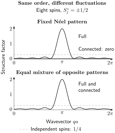
The full structure factor is identical for the two preparations. Subtracting the mean pattern removes the peak only in the fixed product state. The gray reference is an ensemble of independent, equally likely up and down spins, for which both structure factors equal $1/4$. These exact eight-site examples illustrate definitions, not experimental data or a thermodynamic phase transition.

A digital Hubbard experiment: what sixteen qubits measured

Stanisic and collaborators (2022) used 16 superconducting qubits to represent eight spatial sites with two spin modes each. Their $1\times8$ chain and $2\times4$ ladder calculations used a noninteracting initial state, variational hopping and interaction gates, and error mitigation. The measurements reproduced qualitative ground-state features, including density oscillations and antiferromagnetic correlations.

These were finite instances with classical reference calculations. The authors’ extrapolation toward quantitative calculations at larger sizes required much deeper circuits than the demonstrated ones. The experiment thus illustrates how an algorithm exposes many-body observables on hardware; the number of encoded modes alone does not establish a computational speedup.

Postselection also affects the experimental cost. The reported 16-qubit experiments retained approximately 7–29% of runs after checking the occupations of both spin sectors. Obtaining $M$ retained shots then requires about $M/a$ raw shots at acceptance probability $a$, before other calibration or mitigation measurements. This is a mean cost, not a guarantee for a fixed shot budget. Conditioning on the correct particle number removes some errors, but errors within that sector can remain.

For a different task—estimating an eigenvalue to high precision—phase estimation trades measurement repetitions for long coherent evolution. Its usefulness also depends on preparing a state with appreciable weight on the desired eigenstate. The materials simulation guide develops this comparison with variational and analog approaches.

Rydberg arrays: the geometry changes the Hamiltonian

Ebadi and collaborators (2021) studied ordered phases and critical dynamics in programmable arrays with up to 256 Rydberg atoms. The excitation of each atom acts as a two-state degree of freedom. In a common convention,

$$\begin{aligned} H={}&\frac{\hbar\Omega}{2}\sum_i X_i -\hbar\Delta\sum_i n_i +\sum_{i<j}V_{ij}n_in_j,\\ n_i={}&\frac{I+Z_i}{2}. \end{aligned}$$

Here $\Omega$ and $\Delta$ are angular frequencies, while $V_{ij}$ is an energy, approximately $C_6/r_{ij}^6$ in the relevant van der Waals regime. Expanding the interaction gives an Ising coupling $V_{ij}Z_iZ_j/4$ and a longitudinal field coefficient

$$b_i=-\frac{\hbar\Delta}{2} +\frac14\sum_{j\ne i}V_{ij}.$$

Consequently, a uniform laser detuning does not generally produce a uniform effective longitudinal field near an array boundary. Missing atoms and interaction tails also change the model. This matters when comparing an observed pattern with a nearest-neighbor Ising calculation. A pattern produced by a finite-rate ramp need not equal an equilibrium state at a known temperature.

The experiment’s scientific questions concern ordering, fluctuations and dynamics of the implemented Hamiltonian. Mapping those results to a named magnetic material additionally requires matching its low-energy degrees of freedom and couplings.

Kicked-Ising dynamics and an improving classical comparison

Kim and collaborators (2023) measured observables of kicked-Ising circuits on 127 qubits, reaching 60 CNOT layers in the deepest experiments. They used Pauli twirling, learned noise models and probabilistic error amplification followed by zero-noise extrapolation. Amplifying a physical noise channel and extrapolating its effect differs from probabilistic error cancellation, which samples a signed representation of an inverse channel. The paper discussed the latter as an alternative with a different sampling cost.

The ideal target was the discrete circuit itself. For example, a step may be written

$$U_{\mathrm{step}} =e^{-i\alpha\sum_iX_i} e^{-i\beta\sum_{\langle i,j\rangle}Z_iZ_j},$$

with dimensionless angles $\alpha,\beta$. Interpreting repeated steps as continuous evolution under the sum of the two generators introduces a separate product-formula approximation because the generators do not commute. Accurate execution of the circuit does not remove that approximation.

Tindall and collaborators (2024) subsequently used a tensor network adapted to the heavy-hexagon graph and an approximate contraction based on belief propagation. It reproduced the studied observables more accurately and precisely than the quantum estimates. This example shows why a comparison with one unsuccessful classical representation cannot establish that the physical problem itself is beyond classical calculation. The original device measurements and a later improvement in classical computation can both be valid results.

Comparing a model with a real magnetic material

Two 2026 studies make the material connection explicit. Lee and collaborators used up to 50 qubits in a quantum–classical calculation of dynamical structure factors and compared the resulting spectra with neutron-scattering measurements of $\mathrm{KCuF}_3$. Leclerc and collaborators implemented an effective model of the frustrated magnet $\mathrm{TmMgGaO}_4$ on a 256-qubit Rydberg array and compared its magnetization with single-crystal measurements. The cited arXiv versions are research preprints; these examples illustrate the comparison being attempted rather than a general advantage claim.

A scattering spectrum contains more information than a ground-state energy. It resolves correlations in space and time. Comparing it with measured intensity requires the appropriate magnetic form factors, polarization factors, temperature and instrument resolution. The same model can describe one observable well while missing another because it omits disorder, interlayer coupling or higher-energy states.

Finite observation time also broadens a calculated spectrum. For a one-sided rectangular record of duration $T$, a single oscillation at angular frequency $\omega_0$ gives a normalized transform

$$\begin{aligned} A_T(\omega)&=\frac1T\int_0^T e^{i(\omega-\omega_0)t}\,dt,\\ |A_T(\omega)|&=\left|\operatorname{sinc} \frac{(\omega-\omega_0)T}{2}\right|, \end{aligned}$$

where $\operatorname{sinc}x=\sin x/x$. Its first zero lies at $|\omega-\omega_0|=2\pi/T$. This is a window scale, not a universal uncertainty bound on a fitted frequency. Sampling more finely at the same $T$ does not narrow this window; measuring for longer does. Instrument broadening must then be treated consistently when comparing with experiment.

Battery voltage: a property built from several energies

Delgado and collaborators (2022) proposed a fault-tolerant algorithm for battery-material properties and estimated resources for dilithium iron silicate. Their quantum calculation uses first-quantized state preparation and qubitization-based phase estimation. It is a resource study, not a completed battery simulation on hardware.

For a reaction that inserts $\Delta x=x_2-x_1>0$ lithium atoms per formula unit, define the zero-temperature energy difference

$$\begin{aligned} \Delta E&=E_{\mathrm{cath}}(x_2) -E_{\mathrm{cath}}(x_1)-\Delta x E_{\mathrm{Li}},\\ V&=-\frac{\Delta E}{\Delta x e}. \end{aligned}$$

The cathode energies must use the same formula-unit normalization, and $E_{\mathrm{Li}}$ is the reference energy per lithium atom. A negative reaction energy gives a positive voltage. At operating conditions, appropriate free energies and stable phases replace this simple electronic-energy approximation.

For $\Delta x=1$, three independent energy uncertainties of $10\,\mathrm{meV}$ give $\sigma_V=\sqrt3\,(10\,\mathrm{mV})$. With correlated errors, use the covariance of the energy difference. Common errors can cancel between compositions; unrelated systematic model errors do not disappear because quantum measurement noise is small.

Ionic mobility requires further information. On an assumed potential-energy surface, the lowest barrier between specified basins is obtained by minimizing over connecting paths:

$$E_{\mathrm b} =\inf_{\gamma:A\to B}\left[ \max_s E(\gamma(s))-E_A\right].$$

The maximum along an arbitrary chosen path is only an upper bound on this barrier. Even the correct barrier does not alone determine a diffusion coefficient: attempt frequencies, available paths, occupations and temperature also matter. See quantum chemistry case studies for related distinctions between energy accuracy and derived properties.

Exercises

1. Full and connected order

For an even $N$-site chain in a fixed Néel product state, calculate $S^{zz}(\pi/a)$ and $S_c^{zz}(\pi/a)$. Repeat for an equal mixture of the two opposite patterns.

Solution

Every full pair correlation is $G_{jk}=(-1)^{j-k}/4$. At $q=\pi/a$ the Fourier sign cancels this alternating sign, so all $N^2$ terms add:

$$S^{zz}(\pi/a)=\frac{N^2}{4N}=\frac N4.$$

In the fixed pattern, the product of the local means equals $G_{jk}$, giving $S_c^{zz}=0$. In the mixture the means vanish, giving $S_c^{zz}=N/4$. The mixture contains only product states and is separable despite its long-range connected correlations.

2. Independent spins

Each of eight spins independently takes $S_j^z=\pm1/2$ with equal probability. Find both structure factors at every $q$ and compare with the peak in exercise 1.

Solution

The means vanish, distinct-site correlations vanish, and $G_{jj}=C_{jj}=1/4$. Thus both structure factors are $N(1/4)/N=1/4$ at every wavevector. The Néel peak is $8/4=2$, eight times this background. A peak identifies a spatial pattern in correlations; the comparison in exercise 1 shows that it is not by itself an entanglement test.

3. Retained measurements

At acceptance probability $a=0.07$, what is the mean raw-shot cost of collecting 10,000 retained shots? Does that number guarantee 10,000 retained outcomes?

Solution

For independent identical acceptance events, the mean stopping cost is

$$\mathbb E[N_{\mathrm{raw}}]=\frac{10{,}000}{0.07} \approx142{,}857.$$

A fixed budget near the mean does not provide a high-probability guarantee. The retained count at a fixed budget is binomial; a desired confidence level requires its lower tail to be controlled. Particle-number acceptance also does not test every error within the accepted sector.

4. Boundary fields in a Rydberg chain

Take an open three-site chain with nearest-neighbor interaction $V>0$ and no other interactions. Can one uniform detuning make all $b_i$ zero?

Solution

Each end has one neighbor, while the middle site has two:

$$\begin{aligned} b_{\mathrm{end}}&=-\hbar\Delta/2+V/4,\\ b_{\mathrm{middle}}&=-\hbar\Delta/2+V/2. \end{aligned}$$

Their difference is $V/4$ for every uniform detuning. Canceling the end fields leaves a middle field $V/4$. Site-dependent detuning or a different model is needed to cancel all fields.

5. A circuit is not its unsplit Hamiltonian

Starting from $|0\rangle$, compare the final $Z$ expectation under $U=e^{-i\pi X/4}e^{-i\pi Z/4}$ and $W=e^{-i\pi(X+Z)/4}$.

Solution

The rightmost $Z$ rotation in $U$ contributes only a phase to $|0\rangle$. The subsequent $X$ rotation turns the Bloch vector by $\pi/2$, so $\langle Z\rangle_U=0$. The unitary $W$ rotates by $\pi/\sqrt2$ about $(\hat x+\hat z)/\sqrt2$, giving

$$\langle Z\rangle_W =\frac{1+\cos(\pi/\sqrt2)}{2} \approx0.19715.$$

The discrepancy is present even with perfect gates. Reducing the step size at fixed total evolution time controls the product-formula error.

6. Longer time or more samples?

A rectangular record lasts $T=20\hbar/J$. Find the first-zero angular-frequency offset. What happens if the sample count doubles at fixed duration, or the duration doubles?

Solution

$$\delta\omega=\frac{2\pi}{T} =\frac\pi{10}\frac J\hbar.$$

Doubling sample count at fixed duration leaves this offset unchanged, while decreasing the sampling interval and increasing the Nyquist bandwidth. Doubling duration halves the offset. A record from $-T$ to $T$ has duration $2T$ and therefore a first-zero offset $\pi/T$ instead.

7. Correlated voltage errors

For $\Delta x=1$, the two cathode energies each have standard uncertainty $10\,\mathrm{meV}$ and correlation coefficient $0.9$. The lithium reference has independent uncertainty $10\,\mathrm{meV}$. Find $\sigma_V$.

Solution

The covariance of the two cathode energies is $90\,\mathrm{meV}^2$. Because their coefficients have opposite signs,

$$\begin{aligned} \sigma_{\Delta E}^2&=100+100+100-2(90)\\ &=120\,\mathrm{meV}^2. \end{aligned}$$

Thus $\sigma_V=\sqrt{120}\,\mathrm{mV}\approx10.95\,\mathrm{mV}$. This calculation presumes that the stated uncertainties include the errors under discussion; it does not bound an unmodeled bias.

8. A different migration path

Two continuous paths connect the same equal-energy minima. Their energies above either minimum are $E_1(s)=0.8\sin^2(\pi s)\,\mathrm{eV}$ and $E_2(s)=0.3\sin^2(\pi s)\,\mathrm{eV}$ for $0\le s\le1$. What can be concluded about the lowest barrier?

Solution

The path maxima are $0.8$ and $0.3\,\mathrm{eV}$. Considering both proves only $E_{\mathrm b}\le0.3\,\mathrm{eV}$; a third path could be lower. The $0.8\,\mathrm{eV}$ result is a barrier along the first path, not the minimum barrier between the basins.

9. Fit and prediction

Three couplings are fitted to a material’s magnetization curve, which the simulator then reproduces. Give one stronger test of the model and explain its limitation.

Solution

Predict a spectrum or a magnetization curve at unused fields or temperatures, propagating uncertainty in the fitted couplings. Agreement tests predictive behavior beyond the fitting data. It still applies only to the tested regime and observables; it does not establish that every omitted interaction is irrelevant or that the model predicts all material properties.

References

• Delgado, A., et al. “Simulating key properties of lithium-ion batteries with a fault-tolerant quantum computer.” Physical Review A 106, 032428 (2022). doi:10.1103/PhysRevA.106.032428.
• Ebadi, S., et al. “Quantum phases of matter on a 256-atom programmable quantum simulator.” Nature 595, 227–232 (2021). doi:10.1038/s41586-021-03582-4.
• Kim, Y., et al. “Evidence for the utility of quantum computing before fault tolerance.” Nature 618, 500–505 (2023). doi:10.1038/s41586-023-06096-3.
• Leclerc, L., et al. “One-to-one quantum simulation of a frustrated magnet with 256 qubits.” arXiv:2603.20372v3 (2026), preprint. arXiv.
• Lee, Y.-T., et al. “Benchmarking quantum simulation with neutron-scattering experiments.” arXiv:2603.15608v3 (2026), preprint. arXiv.
• Mazurenko, A., et al. “A cold-atom Fermi–Hubbard antiferromagnet.” Nature 545, 462–466 (2017). doi:10.1038/nature22362.
• Stanisic, S., et al. “Observing ground-state properties of the Fermi–Hubbard model using a scalable algorithm on a quantum computer.” Nature Communications 13, 5743 (2022). doi:10.1038/s41467-022-33335-4.
• Tindall, J., Fishman, M., Stoudenmire, E. M., and Sels, D. “Efficient tensor network simulation of IBM’s Eagle kicked Ising experiment.” PRX Quantum 5, 010308 (2024). doi:10.1103/PRXQuantum.5.010308.