Quantum Chemistry Case Studies

Quantum chemistry asks for molecular properties such as binding energies, reaction barriers and spin-state splittings. A quantum processor can help estimate eigenvalues or observables of an encoded electronic Hamiltonian. The scientific question is whether that Hamiltonian, the computed quantity and its accuracy together describe the molecule adequately.

The selected studies below illustrate distinct achievements: small-molecule optimization, accurately executed trial states, logical encoding and conditional estimates for much larger calculations. They are examples with stated dates and assumptions, not a survey of the latest performance.

Required background. Electronic structure introduces orbitals and correlation; quantum chemistry simulation explains the finite Hamiltonian and its encoding. Helpful background. VQE explains variational optimization, while phase estimation explains eigenvalue sampling.

A molecular name does not specify a Hamiltonian

At fixed nuclear geometry, choose a basis and the electronic terms to retain. A complete active space, written CAS($n_{\mathrm e},n_{\mathrm o}$), places $n_{\mathrm e}$ electrons in $n_{\mathrm o}$ selected spatial orbitals. Other orbitals may be frozen or excluded. A direct occupation encoding uses $2n_{\mathrm o}$ qubits before symmetry reductions, because each spatial orbital has two spin states.

For fixed spin-up and spin-down populations, the determinant count is

$$D=\binom{n_{\mathrm o}}{N_\alpha} \binom{n_{\mathrm o}}{N_\beta}.$$

This fixes the spin projection $M_S=(N_\alpha-N_\beta)/2$, not the total spin $S$. In particular, $N_\alpha=N_\beta$ does not make every state a singlet. A calculation targeting a singlet must impose or verify the additional spin condition when relevant.

CAS(6,6) also does not specify which six orbitals were retained. A unitary rotation entirely within a fixed active orbital span leaves its exact full-configuration-interaction result unchanged. Mixing retained and excluded orbitals can change that span and its exact energy. An approximate ansatz can depend on orbital choices even within a fixed span.

For nested many-electron subspaces of the same Hamiltonian, variational ground energies decrease toward the larger-space result. That argument does not automatically apply to different effective Hamiltonians, changed geometries or unrelated downfolding approximations. Keep nuclear and frozen-core constant energy shifts consistent. McArdle and colleagues review how these modeling choices enter quantum chemistry algorithms.

A two-configuration example

Consider an illustrative Hamiltonian in two orthonormal configurations,

$$H=\begin{pmatrix}-1.0&0.2\\0.2&-0.6\end{pmatrix}E_{\mathrm h}.$$

Here $E_{\mathrm h}$ is the hartree; these numbers are chosen for teaching, not fitted to a particular molecule. Retaining only the first configuration gives $-1.0E_{\mathrm h}$. Allowing both gives

$$\begin{aligned} E_0&=(-0.8-\sqrt{0.08})E_{\mathrm h}\\ &\approx-1.08284E_{\mathrm h}. \end{aligned}$$

A perfect one-configuration calculation still misses about $82.8$ millihartree of lowering from configuration mixing. More accurate measurements of the smaller problem cannot remove that difference. This is the basic distinction between solving the chosen model and improving the model or trial space.

Hydrogen: a small problem with an exact reference

Minimal-basis $\mathrm H_2$ has two electrons in two spatial orbitals. Its $M_S=0$ determinant space has dimension four, and further symmetries allow compact circuits. Exact classical diagonalization is easy, which makes it useful for checking an experiment.

O’Malley and colleagues (2016) measured the hydrogen energy curve using superconducting-qubit VQE and a Trotterized phase-estimation implementation. The VQE dissociation-energy error was reported as $(8\pm5)\times10^{-4}E_{\mathrm h}$ relative to the finite-model reference. The one-step Trotter approximation used for phase estimation was insufficient to reach the same accuracy. This tests two implementations at a small scale; it does not establish that VQE remains cheaper as the desired precision and system size change.

The often-used “chemical accuracy” scale of roughly $1\ \mathrm{kcal/mol}$, or $1.6\,\mathrm{m}E_{\mathrm h}$, is a conventional tolerance for energies and energy differences. Whether it suffices depends on the observable. Agreement with a minimal-basis exact result does not include basis-set error relative to the molecule.

Lithium and beryllium hydrides: adapt the circuit to the device

Kandala and colleagues (2017) optimized reduced $\mathrm{LiH}$ and $\mathrm{BeH}_2$ Hamiltonians on superconducting hardware, reaching six-qubit instances. Their trial circuits used native rotations and entangling operations, with stochastic classical optimization. They calibrated and corrected readout assignment errors and compared the observations with device-noise simulations. This paper should not be described as a demonstration of zero-noise extrapolation.

The example shows why short native circuits can be useful while still needing chemical and optimization checks. A circuit with fewer entangling gates may represent the desired state less accurately or explore unwanted particle-number sectors. To distinguish these effects, compare its noiseless optimum with the exact encoded-model energy, then compare the implemented result with that optimum. Gate count alone cannot make those comparisons.

Water: distinguish the prepared states from the complete calculation

Trapped-ion trial states

Nam and colleagues (2020) designed unitary-coupled-cluster circuits for water. Their numerical study reached the finite-basis accuracy target with 17 excitation terms, using a compiled design of 11 qubits and 143 entangling gates.

The experiment measured the first three excitation corrections and scanned small trial-state energy surfaces around numerical optima. It did not execute the entire 17-term optimization on hardware. Those measurements test state preparation, gates and calibrated energy estimation. Distinguishing this result from the larger design makes clear which parts were experimentally checked and which were calculated classically.

Logical states in silicon

Zhang and colleagues (2026) used two logical qubits encoded in a $[[4,2,2]]$ error-detecting code for a reduced water calculation. The selected active space contained two electrons in two orbitals. A classical optimizer updated parameters from logical-state measurements while the bond angle was varied at fixed bond length.

The reported processed energies differed from the paper’s theoretical curve by an average of $22.7\,\mathrm{m}E_{\mathrm h}$. The experiment combined parity checks, Clifford fitting and symmetry verification. It demonstrates an integrated logical-state calculation with detection and mitigation; the small model and residual error do not establish chemical accuracy for full water. A distance-two detection code also does not correct arbitrary unknown single-qubit errors. Acceptance probability and processing choices remain part of the performance description.

Energy curves, differences and forces ask different questions

Define the deviation from a stated reference at geometry $R$ by

$$\Delta(R)=E_{\mathrm{method}}(R)-E_{\mathrm{ref}}(R).$$

A constant offset cancels in energy differences. The nonparallelity error over a specified range,

$$\mathrm{NPE}=\max_R\Delta(R)-\min_R\Delta(R),$$

bounds the error in a difference between any two geometries in that range. A value computed only at sampled geometries need not bound unsampled excursions. Neither a small offset nor a small NPE alone controls derivatives: the force error is $-d\Delta/dR$.

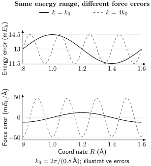
Equal energy-error ranges need not mean equal force accuracy. The illustrative functions are $\Delta(R)=13+1.5\sin[k(R-0.8)]$ in millihartree, with $R$ in ångström. The solid curve uses $k=2\pi/0.8$ and the dashed curve four times that value. Both have NPE $3\,\mathrm{m}E_{\mathrm h}$, but their force-error amplitudes are about $11.8$ and $47.1\,\mathrm{m}E_{\mathrm h}/\text{Å}$. These are calculated examples, not molecular measurements.

Reaction barriers and spin splittings involve subtracting energies. Shared approximations may partly cancel, but that cancellation must be checked across the relevant states and geometries. A tiny statistical error at one geometry cannot establish an accurate dissociation curve or force field.

Cytochrome P450: a resource estimate is conditional

Goings and colleagues (2022) compared classical correlated calculations with fault-tolerant phase-estimation estimates for models of a cytochrome P450 active site.

The study factorized Hamiltonians, estimated non-Clifford operations and compiled scenarios through a surface-code model. Million-qubit, multi-day scenarios describe assumed hardware and particular active-space calculations. They are not observed runtimes. Initial-state overlap also matters: the paper’s timing comparison explicitly omitted repetitions due to potentially small overlap.

Compare the same scientific output. Classical reduced density matrices provide more information than one quantum-computed energy. Additional observables, correlation corrections and state-preparation repetitions can change the comparison. These estimates support sensitivity analysis rather than a hardware forecast.

State overlap and energy resolution

For ideal energy measurement of

$$|\psi\rangle=\sum_j c_j|E_j\rangle,$$

the probability of observing $E_j$ is $|c_j|^2$. Phase estimation approximates this measurement with finite resolution and a chosen energy window. Narrower phase uncertainty cannot reveal a state with zero preparation overlap. An absorption intensity additionally needs a transition matrix element; eigenvalues alone do not give a spectrum with intensities.

Phase estimation develops these mechanisms. Qubitization explains how the Hamiltonian normalization and implemented queries determine cost. When translating logical operations into runtime, use the actual duration of a logical layer, not automatically one physical error-correction cycle. Factories, routing and data dependencies can each limit the schedule; see resource estimation.

These cases suggest a useful sequence of comparisons: validate a small encoded operator, test the algorithm against its exact solution where possible, examine convergence of the chemical model, and compare the complete requested output at matched accuracy and cost. Reporting standards explains which measurements and calculation details make those comparisons interpretable.

Exercises

1. Count determinants, then singlets

For six electrons in six spatial orbitals, find the dimension at $M_S=0$ and the direct occupation-qubit count. For a spin-rotation-invariant problem, obtain the number of singlet states by subtracting the dimension at $M_S=1$.

Solution

There are 12 spin orbitals and therefore 12 occupation qubits before reduction. The two determinant counts are

$$\begin{aligned} D_0&=\binom63\binom63=400,\\ D_1&=\binom64\binom62=225. \end{aligned}$$

Every spin-$S\geq1$ multiplet contributes one state at each of $M_S=0$ and $M_S=1$, while a singlet contributes only at zero. Thus the singlet dimension is $400-225=175$. The 400 determinants are not 400 singlets.

2. Solve the two-configuration model

For the illustrative matrix above, evaluate the energy of $|\psi(\theta)\rangle=\cos\theta|0\rangle-\sin\theta|1\rangle$ and find a minimizing angle.

Solution

$$\frac{E(\theta)}{E_{\mathrm h}} =-0.8-0.2\cos2\theta -0.2\sin2\theta.$$

The last two terms are minimized at $\theta=\pi/8$, giving $-0.8-0.2\sqrt2$. The energy lowering relative to $|0\rangle$ is $0.0828427E_{\mathrm h}$. The calculation tests the trial state against the supplied operator; it does not assign these numbers to real hydrogen.

3. Rotate a basis or change a subspace?

Let $H=\operatorname{diag}(-1,1)E_{\mathrm h}$. Rotate its full two-dimensional basis by an angle $\theta$. Separately, retain only $|v_\theta\rangle=\cos\theta|0\rangle+\sin\theta|1\rangle$. Which ground energy changes?

Solution

The full transformed matrix $U^\dagger HU$ still has eigenvalues $\pm E_{\mathrm h}$. The one-dimensional retained space has energy

$$\langle v_\theta|H|v_\theta\rangle =-\cos(2\theta)E_{\mathrm h}.$$

It changes from $-E_{\mathrm h}$ at zero to zero at $\theta=\pi/4$. A coordinate change within a complete retained space and a change of the retained space are different operations.

4. Compare an offset with curve distortion

At three geometries the energy errors are 12, 15 and 13 millihartree. Find the mean offset, sampled NPE and largest possible error in a difference between those three energies.

Solution

The mean offset is $40/3\approx13.33$ millihartree. The sampled NPE is $15-12=3$ millihartree. For any pair of these points the difference error is $\Delta(R_b)-\Delta(R_a)$, whose absolute value is at most 3 millihartree. No conclusion about unsampled geometries follows without additional information.

5. Check the force errors in the figure

Differentiate its two error curves. Why does their common NPE fail to bound the force error uniformly if the frequency is allowed to increase? What would samples at $R=0.8,1.0,1.2,1.4,1.6$ Å miss?

Solution

For $\Delta=13+1.5\sin[k(R-0.8)]$,

$$\delta F=-1.5k\cos[k(R-0.8)].$$

At $k=2\pi/0.8$ its amplitude is about $11.78$ millihartree per ångström; quadrupling $k$ gives $47.12$. The energy range stays 3 millihartree. Controlling energy variation without controlling how rapidly it varies cannot guarantee accurate derivatives. The stated grid samples the fast curve at integer periods: all five errors are 13 millihartree. Its sampled NPE would be zero despite the variation between samples.

6. Include overlap in repeated phase estimation

The target-eigenstate probability is $p_0=0.25$. Assuming ideal resolution and independent preparations, how many runs give at least a 95% chance of seeing the target once? What if $p_0=0$?

Solution

The miss probability is $0.75^r$. Ten runs leave about $0.0563$ and eleven about $0.0422$, so eleven suffice. If the overlap is zero, no number of these preparations reveals the state. Finite-resolution errors and imperfect preparation would require further analysis.

7. Separate two accuracy improvements

A quantum estimate is $0.8$ millihartree above the exact energy of its active model. A larger nested model lowers the exact energy by $9$ millihartree. What is the original estimate’s discrepancy from the larger-model reference?

Solution

The signed discrepancy is $0.8+9=9.8$ millihartree. The original result has small algorithmic error for its own model, but that does not make it accurate for the enlarged one. Neither model is automatically converged to the physical molecule.

8. Distinguish energies from intensities

A two-level system has fixed energies $E_0,E_1$. Compare an optical transition operator with off-diagonal element $d_{01}=0$ to one with $d_{01}=d\ne0$. Do their eigenvalue lists determine the same absorption line strength?

Solution

No. For an initially occupied lower level and the same driving field, the transition strength is proportional to $|d_{01}|^2$. The first transition is dark in this approximation; the second can be bright. The energy spacing identifies a possible resonance frequency but does not determine its intensity, selection rules or population.

9. Check a runtime bottleneck

A hypothetical energy-estimation circuit consumes $10^8$ resource states from factories supplying a total $10^4$ per second. Its dependency chain contains $3\times10^6$ logical layers, each taking 5 ms. Ignore other costs. Which lower bound is larger?

Solution

Supply alone requires $10^4$ seconds, while the chain requires $1.5\times10^4$ seconds. Runtime is at least the larger value, about 4.17 hours. More factories cannot remove this chain bound. Their overlap in a real schedule determines whether the maximum is achievable; state preparation, routing and repetitions can increase the total.

10. Interpret a logical chemistry demonstration

Why do two encoded qubits with postselected error detection and a reduced molecular objective not by themselves establish a fault-tolerant solution of the full molecule?

Solution

Encoding, error detection, accepted logical performance and model adequacy are separate questions. The demonstration must specify which faults are detected, which operations remain reliable, how often data are accepted and how errors accumulate with circuit size. The selected molecular subspace must also be accurate for the desired observable. Successful execution of the reduced problem can test an important combination of components without establishing those larger claims.

References

• Goings, J. J., White, A., Lee, J., Tautermann, C. S., Degroote, M., Gidney, C., Shiozaki, T., Babbush, R., and Rubin, N. C. “Reliably assessing the electronic structure of cytochrome P450 on today’s classical computers and tomorrow’s quantum computers.” Proceedings of the National Academy of Sciences 119, e2203533119 (2022). doi:10.1073/pnas.2203533119; arXiv:2202.01244.
• Kandala, A., Mezzacapo, A., Temme, K., Takita, M., Brink, M., Chow, J. M., and Gambetta, J. M. “Hardware-efficient variational quantum eigensolver for small molecules and quantum magnets.” Nature 549, 242–246 (2017). doi:10.1038/nature23879.
• McArdle, S., Endo, S., Aspuru-Guzik, A., Benjamin, S. C., and Yuan, X. “Quantum computational chemistry.” Reviews of Modern Physics 92, 015003 (2020). doi:10.1103/RevModPhys.92.015003.
• Nam, Y., et al. “Ground-state energy estimation of the water molecule on a trapped-ion quantum computer.” npj Quantum Information 6, 33 (2020). doi:10.1038/s41534-020-0259-3.
• O’Malley, P. J. J., et al. “Scalable quantum simulation of molecular energies.” Physical Review X 6, 031007 (2016). doi:10.1103/PhysRevX.6.031007.
• Zhang, C., et al. “Universal logical operations in a silicon quantum processor.” Nature Nanotechnology (2026). doi:10.1038/s41565-026-02140-1.