Sensing Case Studies

A quantum sensor converts a field, frequency or acceleration into a change in a quantum state, then infers the quantity from measured outcomes. The useful precision depends on the whole measurement cycle: signal accumulation, decoherence, readout, repetition and calibration. These case studies connect that reasoning to clocks, diamond spins, atom interferometers and Rydberg electrometers.

Required background. Measurement as estimation, Fisher information and Cramér–Rao bounds explain local statistical precision. Helpful background. The standard quantum limit and quantum sensing explain independent probes, coherence and readout.

Ramsey clocks: a longer interrogation is not always better

In a simple Ramsey experiment, the excitation probability is

$$\begin{aligned} P(\phi)&=\frac{1+C\cos\phi}{2},\\ \phi&=2\pi(\nu-\nu_0)T+\phi_c. \end{aligned}$$

Here $T$ is the free-evolution time, $C$ the fringe contrast and $\phi_c$ a controlled phase. At the middle of a fringe, $P=1/2$ and $|\partial P/\partial\phi|=C/2$. For $N$ independent identical atoms, binomial projection noise gives $\Delta P=1/(2\sqrt N)$ and local phase uncertainty $\Delta\phi=1/(C\sqrt N)$.

If independent cycles take time $T_c$, the corresponding projection-noise contribution to fractional frequency instability after averaging for $\tau$ is

$$\sigma_y(\tau)\simeq \frac{1}{2\pi\nu_0CT\sqrt N} \sqrt{\frac{T_c}{\tau}}.$$

This expression assumes operation near the known fringe slope and many cycles. Laser noise, dead-time aliasing, imperfect readout and drift can add other contributions. A narrow fringe does not by itself establish a small frequency uncertainty, and its periodicity makes the inference ambiguous without prior frequency information or additional measurements.

Consider an illustrative contrast decay $C=e^{-T/T_2}$ and dead time $t_d$, so $T_c=T+t_d$. The frequency-uncertainty coefficient then scales as

$$\eta_\nu\propto \frac{\sqrt{T+t_d}}{T}e^{T/T_2}.$$

Initially, longer interrogation accumulates more phase. Eventually the contrast loss outweighs that benefit. Dead time also changes the best choice because each short interrogation still pays the preparation and readout cost.

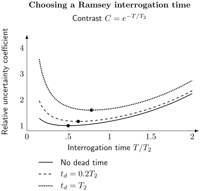
Independent-atom model with exponential contrast decay. All curves use the same normalization: the minimum for zero dead time equals one. Dots mark the optimal interrogation time. Increasing dead time raises the uncertainty and moves the optimum from $T=T_2/2$ toward $T=T_2$. These are illustrative calculations, not fits to a particular clock.

Accuracy requires a separate calculation of frequency shifts. Heavner and collaborators’ first NIST-F2 evaluation (2014) used an approximately 80 K interrogation region to reduce the blackbody-radiation contribution. For the 2013 evaluation they reported Type A and Type B standard uncertainties of $0.44\times10^{-15}$ and $0.11\times10^{-15}$. These labels describe how uncertainty is evaluated—statistical analysis versus other information—not a universal division into random and systematic errors. Reducing statistical fluctuations does not remove an uncertain frequency shift. See atomic clocks for the physical corrections.

Spin squeezing: distinguish a state from a working clock

For collective dimensionless spin with mean along $x$, the Wineland parameter is

$$\xi_R^2=\frac{N(\Delta J_y)^2}{|\langle J_x\rangle|^2}.$$

Small rotations that shift $J_y$ then have local uncertainty $\Delta\phi=\xi_R/\sqrt N$. The denominator already includes the mean-spin contrast. Applying another contrast penalty to this same expression would count that loss twice. An ideal coherent spin state has $\xi_R^2=1$; reduced spin variance alone is insufficient if the signal slope is reduced even more. See spin squeezing for the derivation and entanglement conditions.

Eckner and collaborators (2023) used Rydberg interactions in an optical clock and demonstrated nearly 4 dB of metrological spin squeezing. Their clock comparison reported 1.94(1) dB improvement below its standard-quantum-limit reference, with fractional instability $1.087(1)\times10^{-15}$ at one second. The state characterization and the clock performance are distinct measurements.

Robinson and collaborators (2024) used cavity measurements to prepare squeezed strontium ensembles. Their direct comparison improved from $1.58(3)$ to $1.27(2)$ in units of $10^{-15}(\tau/\mathrm s)^{-1/2}$, a 1.9(2) dB stability improvement without subtracting technical noise. The comparison nevertheless remained above the paper’s effective standard quantum limit. The reference state, contrast and treatment of participating atoms matter when interpreting the benchmark.

A measured variance reduction of $g$ dB means a variance ratio $10^{-g/10}$ and a standard-deviation ratio $10^{-g/20}$. It does not by itself determine $\xi_R^2$. Even an independently measured $\xi_R^2<1$ may fail to improve elapsed-time precision if squeezing greatly lengthens the cycle or if another noise source dominates. With matched atom number and interrogation time, ideal projection-limited variance per averaging time scales as $\xi_R^2T_c$.

Diamond magnetometry: distinguish magnetic shifts from other shifts

For an NV center with a sufficiently axial bias field, a useful approximation to its two electronic-spin transition frequencies is

$$\begin{aligned} \omega_\pm&\simeq D\pm\gamma_eB_z,\\ \frac{\gamma_e}{2\pi}&\simeq28\ \mathrm{GHz/T}. \end{aligned}$$

Here $D$ and $\omega_\pm$ are angular frequencies. Their average estimates $D$, while their difference estimates the axial magnetic field. Temperature can shift $D$, so using both transitions helps separate a common frequency shift from a magnetic one.

The linear model presumes that transverse mixing is negligible and that the chosen hyperfine components are treated consistently. In a simple two-state subspace with transverse mixing $E$, the frequencies instead have the form

$$\omega_\pm=D\pm\sqrt{(\gamma_eB_z)^2+E^2}.$$

Near zero field the splitting is not linear in $B_z$ and loses first-order sensitivity to it. Extrapolating the large-bias calibration to that regime would misidentify the field.

A pulse sequence measures a filtered field through

$$\phi=\gamma_e\int y(t)B_z(t)\,dt,$$

where $y(t)$ changes sign at refocusing pulses. Ramsey interrogation has $y=1$ during free evolution; echo and dynamical-decoupling sequences select different time-dependent signals. A sensitivity for an oscillating field at the sequence’s passband therefore does not describe arbitrary dc fields.

Wolf and collaborators’ ensemble experiment (2015), as corrected in its 2023 erratum, achieved sensitivity $9\,\mathrm{pT}/\sqrt{\mathrm{Hz}}$ and approximately $900\,\mathrm{fT}$ minimum detectable field after 100 s. The originally quoted sensitivity was too optimistic by a factor of ten. This was ensemble ac magnetometry; it does not simultaneously demonstrate the spatial resolution of a shallow single-NV probe. Sensing volume, standoff and frequency response must be matched when comparing the architectures.

An averaging coefficient defined by $\eta_B=\delta B(\tau)\sqrt\tau$ has units $\mathrm T/\sqrt{\mathrm{Hz}}$. Those units alone do not fix its relation to a spectral amplitude density: one-sided versus two-sided spectra and the measurement filter introduce factors. For white one-sided field-noise power spectrum $S_B$ and a simple boxcar average, $\operatorname{Var}(\bar B)=S_B/(2\tau)$, so this coefficient is $\sqrt{S_B/2}$.

Atom gravimeters measure acceleration relative to laser phase fronts

A three-pulse light-pulse interferometer has, in an ideal vertical geometry,

$$\phi=(k_{\mathrm{eff}}g-\alpha_c)T^2+\phi_{\mathrm{sys}}.$$

The pulse spacing is $T$, $k_{\mathrm{eff}}$ is the effective wavevector, and $\alpha_c$ is the applied angular-frequency chirp rate. The chirp tracks the falling atoms and removes a large known phase. The residual phase also depends on mirror motion, rotation, wavefront distortions and other effects collected in $\phi_{\mathrm{sys}}$.

Ménoret and collaborators (2018) demonstrated a transportable gravimeter operating at 2 Hz, with reported sensitivity $500\,\mathrm{nm\,s^{-2}}/\sqrt{\mathrm{Hz}}$ and long-term stability below $10\,\mathrm{nm\,s^{-2}}$. A month-long field deployment illustrated the importance of vibration correction and environmental changes. Precision after averaging is not automatically absolute accuracy: a stable wavefront or alignment bias can remain. The use of matter waves also does not imply entanglement among atoms; the demonstrated signal is compatible with independent-atom interference.

Rydberg electrometry: which frequency axis was scanned?

A resonant electric field couples two Rydberg levels with angular Rabi frequency

$$\Omega=\frac{dE_{\mathrm{pk}}}{\hbar}.$$

The dipole matrix element $d$ includes the polarization projection, and $E_{\mathrm{pk}}$ is the local peak field amplitude. In the resolved, resonant two-level limit, the atomic dressed-state splitting in hertz is $\Delta f_0=\Omega/(2\pi)$, giving $E_{\mathrm{pk}}=h\Delta f_0/d$. For a sinusoid, the rms field is smaller by $\sqrt2$.

Sedlacek and collaborators (2012) used optical electromagnetically induced transparency to read out microwave-induced splittings in a vapor cell, reporting sensitivity of approximately $30\,\mu\mathrm{V/cm}/\sqrt{\mathrm{Hz}}$. The optical spectrum is the measurement, so its frequency axis must be converted correctly to the atomic splitting.

For the counter-propagating thermal-vapor arrangement analyzed by Holloway and collaborators (2014), scanning the probe laser gives

$$\begin{aligned} \Delta f_0&=\frac{\lambda_p}{\lambda_c}\Delta f_p,\\ E_{\mathrm{pk}}&=\frac{h}{d} \frac{\lambda_p}{\lambda_c}\Delta f_p. \end{aligned}$$

Here $\lambda_p,\lambda_c$ are the probe and coupling wavelengths, and $\Delta f_p$ is the measured probe-frequency separation. The wavelength factor comes from Doppler selection. It must not be inserted into a splitting already expressed on the atomic frequency scale. Off resonance, the ideal dressed splitting instead involves $\sqrt{\Omega^2+\delta^2}$, where $\delta$ is angular detuning; a larger splitting can therefore reflect detuning rather than a stronger field. Cell perturbations, polarization, spatial averaging and uncertainty in $d$ also affect inference of an external field. See Rydberg electrometry for the fuller model.

Exercises

1. A projection-noise estimate

Use $\nu_0=9.192631770\,\mathrm{GHz}$, $T=0.5$ s, $C=0.8$, $N=10^6$, $T_c=1.2$ s and $\tau=100$ s. Estimate the projection-noise fractional instability.

Solution

The single-cycle phase uncertainty is $1/(0.8\sqrt{10^6})=0.00125$ rad. Dividing by $2\pi\nu_0T$ and multiplying by $\sqrt{1.2/100}$ gives

$$\sigma_y\simeq4.74\times10^{-15}.$$

This is one contribution under the independent-cycle model. It does not include laser noise or an uncertain systematic frequency shift.

2. Finding the best interrogation time

Set $x=T/T_2$ and $d=t_d/T_2$. Minimize $f(x)=e^x\sqrt{x+d}/x$ for positive $x$. Find the optimum for $d=0$, $0.2$ and $1$.

Solution

Differentiating the logarithm gives

$$\frac{d\ln f}{dx}=1+\frac1{2(x+d)}-\frac1x.$$

Setting this to zero gives $2x^2+(2d-1)x-2d=0$. The positive solution is

$$x_* =\frac{1-2d+\sqrt{(1-2d)^2+16d}}4.$$

The three optima are $0.5$, $0.6217$ and $0.7808$. The uncertainty diverges at both short and long interrogation times in this model, so the stationary point is a minimum. As dead time grows, $x_*\to1$.

3. State squeezing and clock gain

A clock comparison improves by 1.94 dB in variance. Find its variance and standard-deviation ratios. Separately, a state has $\xi_R^2=0.5$ but triples the cycle time at fixed $N$ and $T$. Does it improve ideal precision per elapsed time?

Solution

The clock ratios are $10^{-1.94/10}\simeq0.6397$ and $10^{-1.94/20}\simeq0.7998$. These measured ratios do not determine the state’s Wineland parameter without additional information. In the second example, the variance ratio per averaging time is $0.5\times3=1.5$: the longer cycle outweighs the state improvement.

4. Rejecting a common frequency shift

Two NV transitions each have frequency uncertainty $\sigma$, with correlation coefficient $\rho$. In the linear axial model, what is the variance of $B_z=(\omega_+-\omega_-)/(2\gamma_e)$? Why can the same formula fail near a transverse avoided crossing?

Solution

$$\operatorname{Var}(B_z) =\frac{\sigma^2(1-\rho)}{2\gamma_e^2}.$$

Positively correlated common shifts cancel in the difference; independent errors give $\rho=0$. Near the avoided crossing the splitting is $2\sqrt{(\gamma_eB_z)^2+E^2}$, not $2\gamma_eB_z$. At zero field its first derivative vanishes, so the linear calibration and its uncertainty formula no longer apply.

5. Averaging and spectral conventions

Assume an averaging coefficient of $9\,\mathrm{pT}\sqrt{\mathrm s}$ remains white for 100 s. What uncertainty follows? If that coefficient came from a boxcar average of white noise, what one-sided spectral amplitude density would correspond to it?

Solution

The uncertainty is $9/\sqrt{100}=0.9$ pT, or 900 fT. Under the explicitly stated boxcar convention, the one-sided amplitude density is $\sqrt2\times9\simeq12.73\,\mathrm{pT}/\sqrt{\mathrm{Hz}}$. The numerical conversion should not be imposed on a published sensitivity without checking how that paper defines its estimator and bandwidth.

6. Gravity phase and a small change

Take $k_{\mathrm{eff}}=4\pi/(780\,\mathrm{nm})$, $T=60$ ms and $g=9.81\,\mathrm{m/s^2}$. Find the unchirped phase and the phase change for $\delta g=10^{-8}\,\mathrm{m/s^2}$.

Solution

$$\begin{aligned} k_{\mathrm{eff}}gT^2&\simeq5.69\times10^5\ \mathrm{rad},\\ k_{\mathrm{eff}}\delta gT^2&\simeq5.80\times10^{-4}\ \mathrm{rad}. \end{aligned}$$

The applied chirp largely cancels the first quantity. Resolving the second requires a residual-phase measurement near 0.58 mrad as well as control of systematic phases; it is not obtained by reading a large uncalibrated fringe count.

7. A probe-scan conversion

Let $d=1000ea_0$, $\lambda_p=780$ nm, $\lambda_c=480$ nm and measured probe splitting $\Delta f_p=1$ MHz in the stated thermal-vapor geometry. Find the atomic splitting and local peak field. Use $ea_0=8.47835\times10^{-30}\,\mathrm{C\,m}$.

Solution

The atomic splitting is $(780/480)(1\,\mathrm{MHz})=1.625$ MHz. The dipole magnitude is $d=8.47835\times10^{-27}\,\mathrm{C\,m}$, so

$$\begin{aligned} E_{\mathrm{pk}}&=\frac{h(1.625\times10^6\,\mathrm{s^{-1}})}d\\ &\simeq0.127\ \mathrm{V/m}. \end{aligned}$$

Using 1 MHz directly would give about $0.0782\,\mathrm{V/m}$ and miss the scan-axis factor. If the supplied 1 MHz had already been the atomic splitting, that latter result would instead be appropriate.

8. Detuning and rms amplitude

An ideal dressed-state splitting is 5 MHz and the RF detuning is 3 MHz, both expressed in cycles per second. What is $\Omega/(2\pi)$? How does the inferred rms field compare with using the full 5 MHz as a resonant peak-field estimate?

Solution

The resonant coupling frequency is $\sqrt{5^2-3^2}=4$ MHz. The actual peak field is therefore $4/5$ of the naive peak estimate; the rms field is $4/(5\sqrt2)\simeq0.5657$ of that estimate. Both corrections require the stated two-level and sinusoidal-field assumptions.

9. Local precision does not locate the fringe

A Ramsey measurement at time $T$ has excellent local phase precision. Can it distinguish frequency offsets $\Delta\nu$ and $\Delta\nu+1/T$ using that same excitation probability alone?

Solution

No. Their phases differ by $2\pi$, giving the same probability. A prior range, a coarse measurement, or additional interrogation times can resolve the ambiguity. The local Fisher information describes the slope within an identified fringe, not global uniqueness of the frequency estimate.

References

• Eckner, W. J., et al. “Realizing spin squeezing with Rydberg interactions in an optical clock.” Nature 621, 734–739 (2023). doi:10.1038/s41586-023-06360-6.
• Heavner, T. P., et al. “First accuracy evaluation of NIST-F2.” Metrologia 51, 174–182 (2014). doi:10.1088/0026-1394/51/3/174.
• Holloway, C. L., et al. “Broadband Rydberg atom-based electric-field probe for SI-traceable, self-calibrated measurements.” IEEE Transactions on Antennas and Propagation 62, 6169–6182 (2014). doi:10.1109/TAP.2014.2360208.
• Ménoret, V., et al. “Gravity measurements below $10^{-9}g$ with a transportable absolute quantum gravimeter.” Scientific Reports 8, 12300 (2018). doi:10.1038/s41598-018-30608-1.
• Robinson, J. M., et al. “Direct comparison of two spin-squeezed optical clock ensembles at the $10^{-17}$ level.” Nature Physics 20, 208–213 (2024). doi:10.1038/s41567-023-02310-1.
• Sedlacek, J. A., et al. “Microwave electrometry with Rydberg atoms in a vapour cell using bright atomic resonances.” Nature Physics 8, 819–824 (2012). doi:10.1038/nphys2423.
• Wineland, D. J., Bollinger, J. J., Itano, W. M., Moore, F. L., and Heinzen, D. J. “Spin squeezing and reduced quantum noise in spectroscopy.” Physical Review A 46, R6797–R6800 (1992). doi:10.1103/PhysRevA.46.R6797.
• Wolf, T., et al. “Subpicotesla diamond magnetometry.” Physical Review X 5, 041001 (2015). Original article; corrected by Physical Review X 13, 029903 (2023), erratum.