Negative Results and Limitations

A limitation is useful when it tells us which route is blocked and why. A theorem can exclude a whole class of methods under precise assumptions. An experiment can constrain an effect within its sensitivity. A better classical algorithm can remove an earlier computational separation. These conclusions have different meanings, and none should be expanded into a verdict on all quantum technology.

Helpful background. Evaluating quantum claims explains task matching and uncertainty. Lower bounds and limitations develops formal resource bounds; this page connects them to experiments and practical calculations.

The assumptions are part of an impossibility result

Unstructured search. Finding one marked item among $N$ possibilities requires $\Omega(\sqrt N)$ quantum oracle queries for bounded-error success in the black-box model. Grover search attains that order. The result does not say every search problem requires that many operations: algebraic structure, promises, or different data access can define a different problem. It also does not turn a quadratic query improvement into a measured runtime advantage. Bennett et al. (1997)

Transversal gates. Eastin–Knill rules out a universal set of transversal encoded unitaries for a nontrivial exact code on finitely many finite-dimensional subsystems that detects arbitrary errors on each individual subsystem. Transversal operations avoid coupling qubits within one block, which helps contain faults. Their limitation motivates additional mechanisms, including code switching and magic-state-assisted gates; it does not prohibit universal fault-tolerant computation. Eastin and Knill (2009) See fault-tolerant gates for the construction details.

A direct optical channel. For a memoryless bosonic pure-loss channel with transmissivity $\eta$, unlimited two-way classical communication and no input-energy constraint, the secret-key capacity is

$$K(\eta)=-\log_2(1-\eta)$$

bits per optical mode use. At high loss it is approximately $\eta/\ln2$. This is an ideal repeaterless capacity, not the achieved key rate of a particular instrument. Intermediate stations or a different channel geometry change the network being compared; they do not falsify the point-to-point theorem. Pirandola et al. (2017)

A repeater can improve on a practical direct implementation while still falling below this ideal bound. Surpassing the correctly normalized bound establishes a stronger result: performance unavailable to any direct protocol within its assumptions. Network case studies explains why memories, timing, and channel-use conventions matter.

No resolved difference is not the same as equivalence

Let $\Delta$ be a candidate method’s improvement over a reference, with positive values meaning better performance. An interval containing zero means the data have not resolved the sign at that confidence level. It does not mean the true improvement is zero.

Before looking at the result, choose a practically meaningful margin $m>0$. An interval entirely inside $(-m,m)$ supports a small-difference conclusion at the stated level and under the statistical model. An interval extending far outside those margins may leave both substantial benefit and substantial harm plausible.

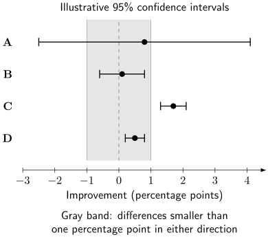
Illustrative 95% intervals, not experimental data. The gray band is the prespecified range $(-1,1)$ percentage points. A is too broad to resolve practical equivalence. B and D lie within the band. C indicates improvement beyond the chosen margin. D excludes zero yet remains practically small: statistical difference and practical equivalence can coexist.

For the standard two-one-sided-tests equivalence procedure at significance level $\alpha$, the matching two-sided confidence interval has level $1-2\alpha$. Thus a 5% equivalence test commonly uses a 90% interval. Requiring the whole 95% interval to lie inside the margins, as in the illustration, is a more conservative criterion. The margin must come from the scientific task, not be widened afterward to fit the observed interval. Lakens (2017)

Uncertainty must include the variation relevant to the claim. Many shots on one circuit do not establish behavior across problem instances. Detector saturation, drift, a poorly calibrated method, or a test set where both methods always succeed can conceal a difference. A useful null result states what effect sizes the experiment could have distinguished.

A faster subroutine can leave the calculation slow

Suppose a fraction $f$ of a serial baseline runtime is accelerated by a factor $S_q$, while all other stages remain unchanged. The total speedup is

$$S=\frac{1}{(1-f)+f/S_q}.$$

At $f=0.20$ and $S_q=100$, the total speedup is only $1.247$. Even an infinitely fast subroutine would give $1.25$, corresponding to a 20% reduction in runtime. Data preparation, repeated measurements, and verification can dominate the rest.

The expression assumes that the new method introduces no additional cost. If its extra preparation takes a fraction $h$ of the original total time, add $h$ to the denominator. With $h=0.30$ in the same example, $S=1/1.102\approx0.907$: the complete calculation is slower. Overlap and parallelism require a different schedule, rather than simply omitting stages.

Probabilistic success adds another cost. For independent identically distributed attempts with success probability $p>0$, finite mean attempt time $\overline t$, and a recognizable success condition,

$$\mathbb E[T_{\rm success}]=\frac{\overline t}{p}.$$

This allows an attempt’s duration to depend on its own outcome, but assumes successive attempts follow the same joint distribution. Drift, timeouts, or exhausted resources can invalidate that model. A heralded operation’s short duration is not its mean delivered latency.

Reducing bias can increase sampling cost

Consider the linear estimator $\widehat\mu=1.5\widehat\mu_1-0.5\widehat\mu_2$. If independent samples in each group have the same variance $\sigma^2$, then

$$\operatorname{Var}(\widehat\mu) =\frac{2.25\sigma^2}{N_1} +\frac{0.25\sigma^2}{N_2}.$$

With a fixed total $N=N_1+N_2$, equal allocation gives $5\sigma^2/N$. Allocating three times as many shots to the first group gives $4\sigma^2/N$, the minimum under these assumptions. Both exceed the variance $\sigma^2/N$ of one equally noisy unmitigated mean. The relevant comparison includes residual bias through mean-squared error, $\mathrm{MSE}=\mathrm{bias}^2+\mathrm{variance}$.

This finite example is distinct from a general lower bound. Takagi and colleagues proved sampling-overhead constraints for broad mitigation protocols, including exponential growth with depth for layered circuits with local depolarizing noise at fixed target accuracy. That result does not assign the same cost to every observable or every structured circuit. Takagi et al. (2022) Limits of error mitigation states the hypotheses more fully.

Three ways a proposed advantage can narrow

The classical input model changes the comparison

Tang’s recommendation algorithm uses a classical data structure supporting length-squared sampling. Under assumptions comparable to the quantum proposal’s input access, the classical method removes the proposed exponential separation, with polynomial dependence on other parameters. This does not make all machine-learning tasks easy: the data structure, approximation rank, accuracy, and output being sampled matter. Tang (2019) See quantum machine learning for the distinction between classical and quantum input data.

A better simulator exploits structure

Tindall and colleagues developed a geometry-aware tensor-network method for the 127-qubit kicked-Ising experiment. It produced more accurate and precise classical observable estimates in the studied setting than the quantum results and several earlier classical methods. Tree-like correlations made the approximation effective. A comparison with the earlier methods therefore could not establish that those observables were beyond classical computation. The experimental measurements remain measurements; what changes is their computational comparison. Tindall et al. (2024)

A similar distinction matters in chemistry. Lee and colleagues examined the case for a generic exponential advantage in ground-state chemistry and found it unestablished. Efficient state preparation and a precise definition of chemically relevant instances are central. That conclusion does not exclude advantages for particular families, different observables, or different scaling regimes. Lee et al. (2023)

An easier training landscape can still be easy to simulate

Trainability and computational advantage are separate. Mele and colleagues studied circuit ensembles with local nonunitary noise and random local gates forming unitary 2-designs. For local-observable costs, their non-unital-noise result avoids the same barren-plateau behavior found in common unital models. Yet typical observable estimates become effectively shallow and admit efficient classical estimation at constant additive accuracy. These are ensemble-dependent statements about expectation values, not a worst-case simulation theorem for every noisy circuit or a guarantee about sampling its full output. Mele et al. (2026)

Structured circuits, altered noise models, and different tasks must be assessed on their own. The variational algorithms and QAOA pages explain how depth, locality, initialization, and sampled gradients enter such comparisons.

A limitation can leave a useful improvement

In many metrology models with fixed independent noise on each probe, asymptotic precision returns to order $N^{-1/2}$ even with entangled inputs, while a constant-factor gain remains possible. The channel, parameter encoding, and resource count determine the bound; correlated noise or error-corrected protocols require their own analysis. Demkowicz-Dobrzański et al. (2012) A constant-factor gain may be valuable for a real sensor even when it changes no scaling exponent.

Likewise, a logical memory can improve without yet providing a complete fault-tolerant computation, and a finite-size quantum simulation can be scientifically useful without outperforming classical methods. State the tested regime, the comparison, and the remaining question. “No improvement was resolved at this precision” and “this theorem forbids the proposed construction” are different scientific results. Error-correction case studies and sensing case studies provide concrete examples.

Exercises

1. Interpret an interval

A relative speed improvement has estimate $0.8\%$ and 95% interval $[-2.5\%,4.1\%]$. The chosen practical margin is one percentage point. Does this show equality, equivalence, or meaningful improvement?

Solution

None of those conclusions follows. The interval includes zero and extends outside both practical margins. It is consistent with meaningful improvement, meaningful harm, and a small difference. The result is inconclusive at the achieved precision. A confidence interval is not a posterior probability distribution over these possibilities.

2. A small but resolved difference

A 95% interval is $[0.2,0.8]$ percentage points, with the same practical margin. Can it exclude zero while supporting practical equivalence?

Solution

Yes. It excludes zero but lies wholly inside $(-1,1)$. A nonzero difference can be too small to matter for the stated task. The usual nested 90% interval would also lie inside the margins and pass the corresponding 5% two-one-sided equivalence test. This conclusion assumes valid intervals and a prespecified margin.

3. Find the runtime bottleneck

Only 20% of a 100-second calculation is accelerated, by a factor of 100. Compute the new runtime, first without extra costs and then with 30 seconds of new state preparation.

Solution

The unchanged work takes 80 seconds and the accelerated work takes $20/100=0.2$ seconds. Totals are therefore 80.2 seconds and 110.2 seconds. Speedups are $1.247$ and $0.907$, respectively. A hundredfold improvement of the selected stage does not specify the whole calculation’s performance.

4. Mean waiting time is not a deadline

Independent attempts take $4\,\mathrm{ms}$ and succeed with probability $0.002$. Find the mean waiting time and the probability of at least one success within 500 attempts.

Solution

The mean is $4\,\mathrm{ms}/0.002=2\,\mathrm{s}$. The deadline is also two seconds, but its success probability is only

$$1-(1-0.002)^{500}\approx0.6325.$$

A mean is not a high-confidence completion time. Fixed attempt duration and independent stationary success are essential to this calculation.

5. Allocate a fixed shot budget

For the estimator above, use $N_1=xN$ and $N_2=(1-x)N$. Minimize its variance for fixed $N$ and explain what remains unknown about its accuracy.

Solution

Apart from $\sigma^2/N$, minimize $2.25/x+0.25/(1-x)$. Setting its derivative to zero gives

$$\frac{1.5}{x}=\frac{0.5}{1-x}, \qquad x=\frac34.$$

The minimum variance is $4\sigma^2/N$. This allocation assumes equal per-shot variances and costs, independent groups, and no uncertainty in the coefficients. The residual bias is still needed to calculate mean-squared error; a lower variance alone does not establish the best estimator.

6. Scope the transversal-gate restriction

Does the Eastin–Knill theorem imply that universal fault-tolerant computation is impossible?

Solution

No. It restricts universal transversal encoded unitaries for the stated fixed exact code. Magic-state-assisted gates and code switching add mechanisms outside that restricted gate set. Their faults and resource costs must still be controlled. Ordinary Clifford-only lattice surgery by itself is not a universal gate set; it also needs a non-Clifford resource or another appropriate extension.

7. A repeater below the ideal bound

For $\eta=10^{-4}$, estimate the ideal direct-channel capacity. A repeater delivers $10^{-5}$ secret bits per consistently counted channel use, while a practical direct implementation delivers $10^{-6}$. What comparison has it won?

Solution

The capacity is approximately $10^{-4}/\ln2=1.4427\times10^{-4}$ bits per mode use. The repeater outperforms the stated practical implementation by a factor of ten, but remains below the ideal direct capacity. It has not exceeded every possible direct protocol. A meaningful comparison must also match trust assumptions and explain how uses of multiple elementary channels are counted.

8. An improved classical calculation

A new classical method estimates a quantum experiment’s target observable more accurately than the earlier classical comparison. Does that invalidate the experimental data or establish that all similar quantum simulations are easy?

Solution

Neither follows. It revises the comparison for the demonstrated task and regime. The new method may depend on special geometry, time scales, or correlations. The original data remain subject to their original measurement uncertainty and calibration checks; computational difficulty is a separate question.

References

• C. H. Bennett, E. Bernstein, G. Brassard, and U. Vazirani, “Strengths and weaknesses of quantum computing,” SIAM Journal on Computing 26, 1510–1523 (1997). doi:10.1137/S0097539796300933.
• R. Demkowicz-Dobrzański, J. Kołodyński, and M. Guţă, “The elusive Heisenberg limit in quantum-enhanced metrology,” Nature Communications 3, 1063 (2012). doi:10.1038/ncomms2067.
• B. Eastin and E. Knill, “Restrictions on transversal encoded quantum gate sets,” Physical Review Letters 102, 110502 (2009). doi:10.1103/PhysRevLett.102.110502.
• D. Lakens, “Equivalence tests: A practical primer for t tests, correlations, and meta-analyses,” Social Psychological and Personality Science 8, 355–362 (2017). doi:10.1177/1948550617697177.
• S. Lee et al., “Evaluating the evidence for exponential quantum advantage in ground-state quantum chemistry,” Nature Communications 14, 1952 (2023). doi:10.1038/s41467-023-37587-6.
• A. A. Mele et al., “Noise-induced shallow circuits and the absence of barren plateaus,” Nature Physics 22, 751–756 (2026). doi:10.1038/s41567-026-03245-z.
• S. Pirandola, R. Laurenza, C. Ottaviani, and L. Banchi, “Fundamental limits of repeaterless quantum communications,” Nature Communications 8, 15043 (2017). doi:10.1038/ncomms15043.
• R. Takagi, S. Endo, S. Minagawa, and M. Gu, “Fundamental limits of quantum error mitigation,” npj Quantum Information 8, 114 (2022). doi:10.1038/s41534-022-00618-z.
• E. Tang, “A quantum-inspired classical algorithm for recommendation systems,” in Proceedings of STOC 2019, 217–228 (2019). doi:10.1145/3313276.3316310.
• J. Tindall, M. Fishman, E. M. Stoudenmire, and D. Sels, “Efficient tensor network simulation of IBM’s Eagle kicked Ising experiment,” PRX Quantum 5, 010308 (2024). doi:10.1103/PRXQuantum.5.010308.